Multi Criteria Overlay Analyse (QGIS3)

Multi-criteria gewogen overlay-analyse is het proces van het toewijzen van gebieden op basis van een variëteit aan eigenschappen die de geselecteerde gebieden zouden moeten hebben. Hoewel dit een veel voorkomende bewerking in GIS is, wordt die het beste uitgevoerd in de rasterruimte met een op een raster gebaseerde benadering.

Notitie

Vector- vs Raster-overlays

U kunt de overlay-analyse uitvoeren op vectorlagen met gereedschappen voor geoverwerking, zoals buffer, dissolve, difference en intersection. Deze methode is ideaal als u een binair antwoord geschikt/niet-geschikt zoekt en u werkt met een handjevol lagen. U kunt onze videohandleiding bekijken op Locating A New Bicycle Parking Station using Multicriteria Overlay Analysis voor een stap-voor-stap gids voor deze benadering.

Werken in de rasterruimte geeft u een rangschikking van de geschiktheid - niet alleen de meest geschikte plek. Het stelt u ook in staat elke aantal invoerlagen gemakkelijk te combineren en verschillende wegingen toe te wijzen aan elk criterium. Over het algemeen is dit de voorkeursbenadering voor geschiktheid.

Deze handleiding gaat door de typische werkstroom voor het uitvoeren van een geschikte plaats-analyse - converteren van bron vectorgegevens naar toepasselijke rasters, ze opnieuw te classificeren en rekenkundige bewerkingen uitvoeren.

Overzicht van de taak

In deze handleiding zullen we de geschikte gebieden voor ontwikkeling identificeren, dat zijn

• Dichtbij wegen en

• Niet in de buurt van watergebieden en

• Niet in een beschermde regio.

De gegevens ophalen

We zullen vector gegevenslagen gebruiken van OpenStreetMap (OSM). OSM is een globale database van vrij beschikbare basis kaartgegevens. Geofabrik verschaft dagelijks bijgewerkte Shapefiles voor gegevenssets van OpenStreetMap.

We zullen de gegevenslagen van OSM gebruiken voor de staat Assam in India. Geofabrik India shapefiles werden gedownload, opnieuw geprojecteerd naar een projectie UTM, geclipt tot de staatsgrenzen en verpakt in één enkel bestand voor GeoPackage. U kunt een kopie van het GeoPackage downloaden vanaf de link hieronder:

assam.gpkg

Gegevensbron: [GEOFABRIK]

Procedure

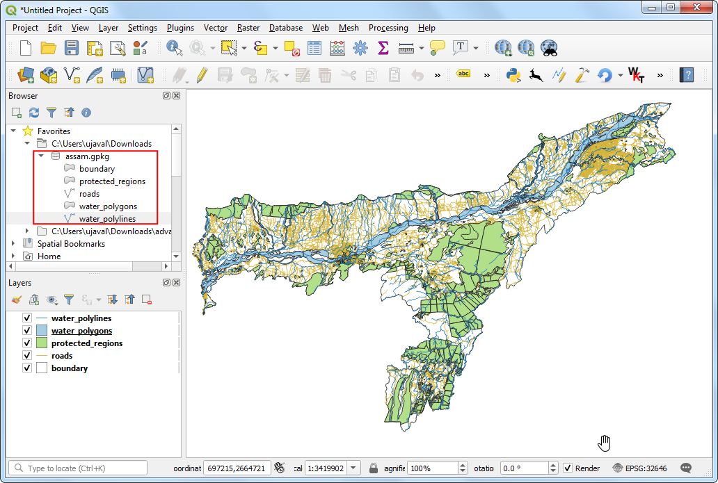
1. Blader naar het gedownloade bestand assam.gpkg in QGIS Browser. Vergroot het en sleep elk van de 5 individuele gegevenslagen naar het kaartvenster. U zult de lagen boundary, roads, protected_regions, water_polygons en water_polylines zien geladen in het paneel Lagen.

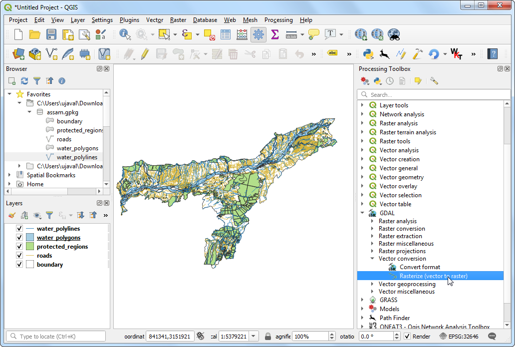
2. De eerste stap in de overlay-analyse, is om elke gegevenslaag te converteren naar een raster. Een belangrijke overweging is dat alle rasters hetzelfde bereik moeten hebben. We zullen de laag boundary gebruiken als het bereik voor alle rasters. Ga naar Processing ‣ Toolbox. Zoek naar en lokaliseer het algoritme GDAL ‣ Vector conversie ‣ Rasteriseren (vector naar raster). Dubbelklik er op om het te starten.

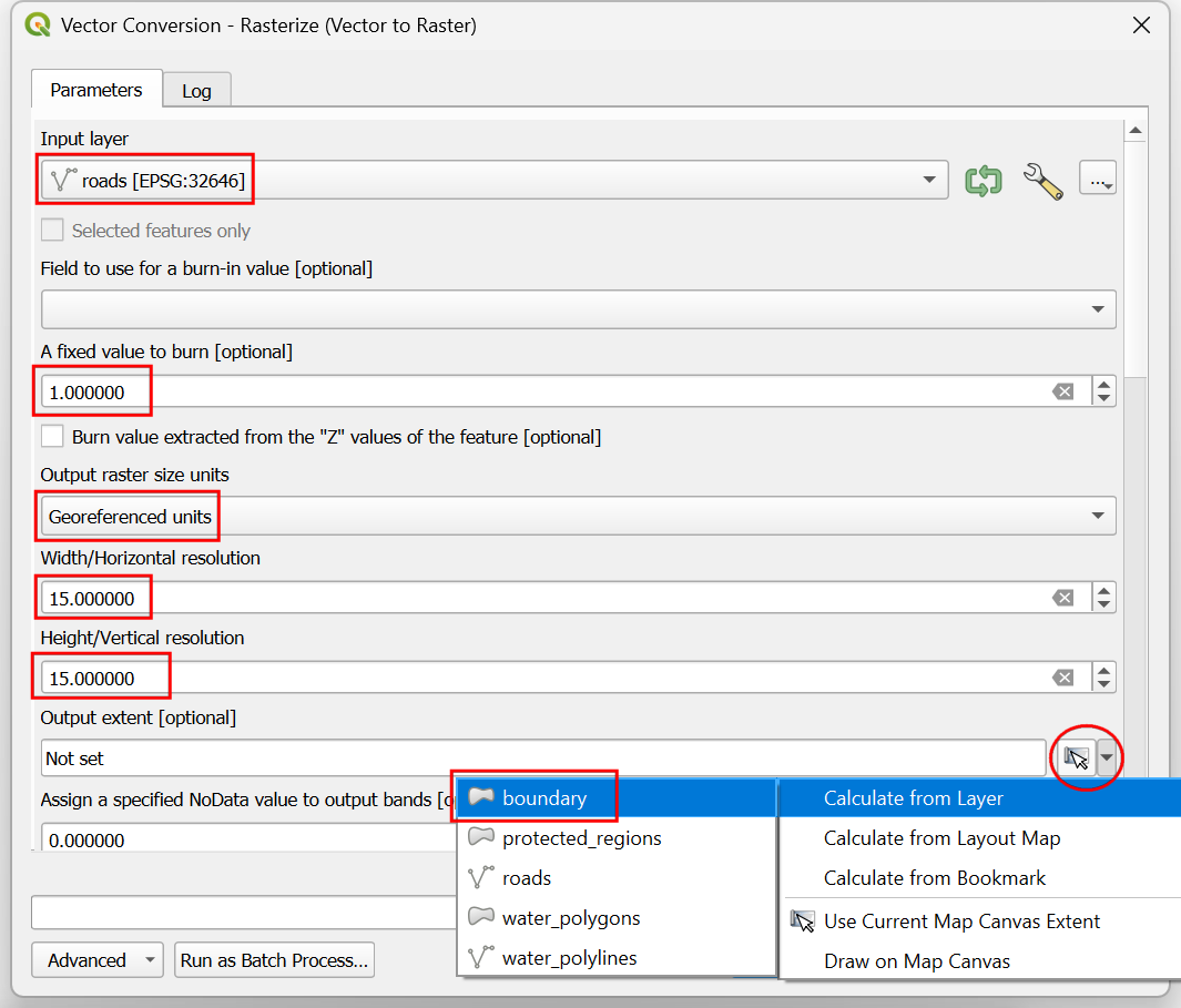
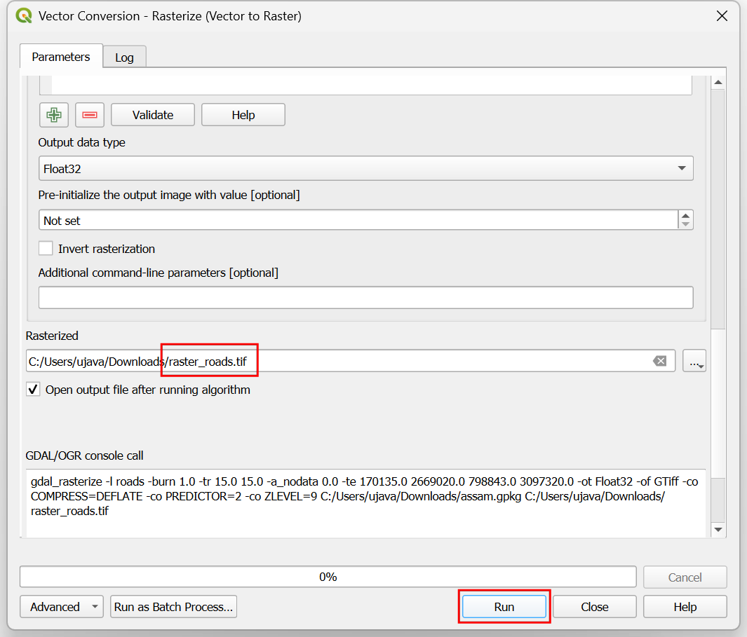
3. In het dialoogvenster Vector conversie - Rasteriseren (vector naar raster), selecteer roads als de Invoerlaag. We willen een uitvoerraster maken met een pixelwaarde van 1 waar een weg is en 0 waar geen wegen zijn. Voer 1 in als de Een vaste waarde om te branden. De invoerlagen zijn in een geprojecteerd CRS met meters als de eenheid. Selecteer Eenheden voor geoverwijzingen als de Eenheden grootte uitvoerraster. We zullen de resolutie van het uitvoerraster instellen op 15 meters. Selecteer 15 voor zowel Breedte/Horizontale resolutie als Hoogte/Verticale resolutie. Klik vervolgens op de pijl naast Bereik uitvoer en selecteer voor Uit laag berekenen ‣ boundary.

4. Scroll naar beneden naar de Geavanceerde parameters en selecteer het profiel Hoge compressie om de compressie toe te passen. Dit zal het gecomprimeerde rasterbestand kleiner maken na het uitvoeren van het gereedschap. Toepassen van compressie zonder verlies wordt enorm aanbevolen bij het werken met rastergegevens.

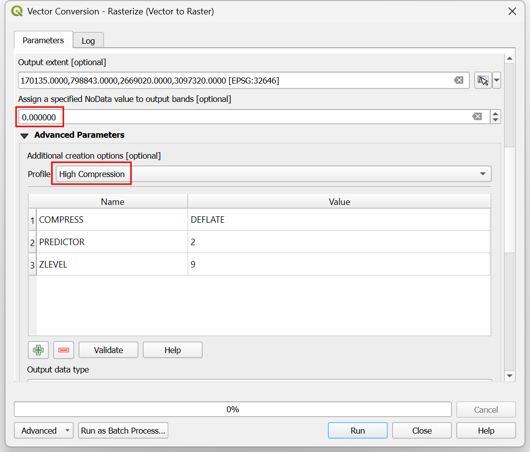
5. Stel het uitvoerraster Gerasteriseerd in als raster_roads.tif en klik op Uitvoeren.

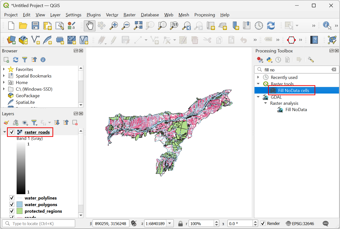
6. Als de verwerking is voltooid zult u een nieuwe laag raster_roads zien geladen in het paneel Lagen. Het raster heeft pixelwaarden 1 voor pixels die kruisen met de wegen. Alle andere pixels zijn ingesteld als waarden Geen gegevens. Deze waarden Geen gegevens zijn problematisch. Als rasterberekeningen (die we later zullen gebruiken) een pixel met een waarde Geen gegevens tegenkomt in enige laag, stelt het ook de waarde voor de uitvoer van die pixel in als Geen gegevens, wat dus onverwachte uitvoer geeft. We zullen deze waarden vullen met de waarde 0. Zoek naar en lokaliseer het algoritme Raster-gereedschappen ‣ Cellen met Geen gegevens vullen. Dubbelklik erop om het te starten.

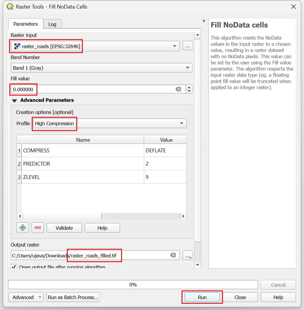
7. Selecteer raster_roads als de Raster input en kies 0 als de Vulwaarde. Scroll naar beneden naar de Geavanceerde parameters en selecteer het profiel Hoge compressie om de compressie toe te passen. Stel het uitvoerbestand in op roads_proximity.tif en klik op Uitvoeren.

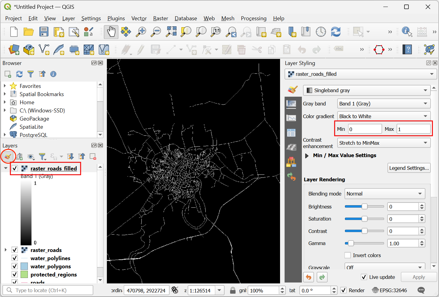
8. Als de verwerking eenmaal is voltooid, zult u de nieuwe laag raster_roads_filled zien geladen in het paneel Lagen. Dit raster heeft de waarden 1 voor wegen en 0 voor niet-wegen. Als de laag niet correct wordt gevisualiseerd, kunt u klikken op de knop Paneel Laag opmaken openen en de Min instellen op 0 en Max op 1.

9. Herhaal de stappen 3-8 voor de andere 3 vectorlagen protected_regions, water_polylines en water_polygons. U moet deze lagen rasteriseren en de cellen met Geen gegevens vullen. Als u deze stappen handmatig wilt uitvoeren, kunt u het dialoogvenster voor het uitvoieren van het algortime configureren, het algoritme ujitvoeren en als het algoritme eenmaal is voltooid, schakelen naar de tab Parameters en eenvoudigweg de namen voor invoer- en uitvoerlagen wijzigen. U kunt ook elk algoritme over alle 4 lagen in een stap uitvoeren met Batch Processing. Bekijk de handleiding Massa verwerken met behulp van Framework Processing (QGIS 3) om daar meer over te weten te komen. Als u eenmaal klaar bent, zou u 4 rasterlagen moeten hebben en de volgende corresponderende rasterlagen moeten maken raster_roads_filled, raster_protected_regions_filled, raster_water_polylines_filled en raster_water_polygons_filled. Het zal u opvallen dat we 2 aan water gerelateerde lagen hebben - beide geven water weer. We kunnen ze samenvoegen tot een enkele laag die de watergebieden in de regio weergeeft. Zoek naar en lokaliseer het algortime Raster analysis ‣ Rastercalculator in de Toolbox van Processing. Dubbelklik eorp om het te starten.

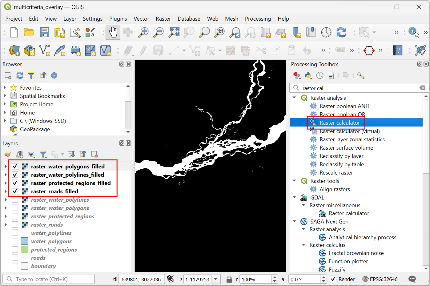
10. Selecteer de lagen raster_water_polygons en raster_water_polylines met de knop … als Invoerlagen. Voer de volgende expressie in met de knop ε. Laat alle andere opties als standaard staan en sla de uitvoerlaag op met de naam raster_water_merged.tif en klik op Uitvoeren.

"raster_water_polygons_filled@1" + "raster_water_polylines_filled@1"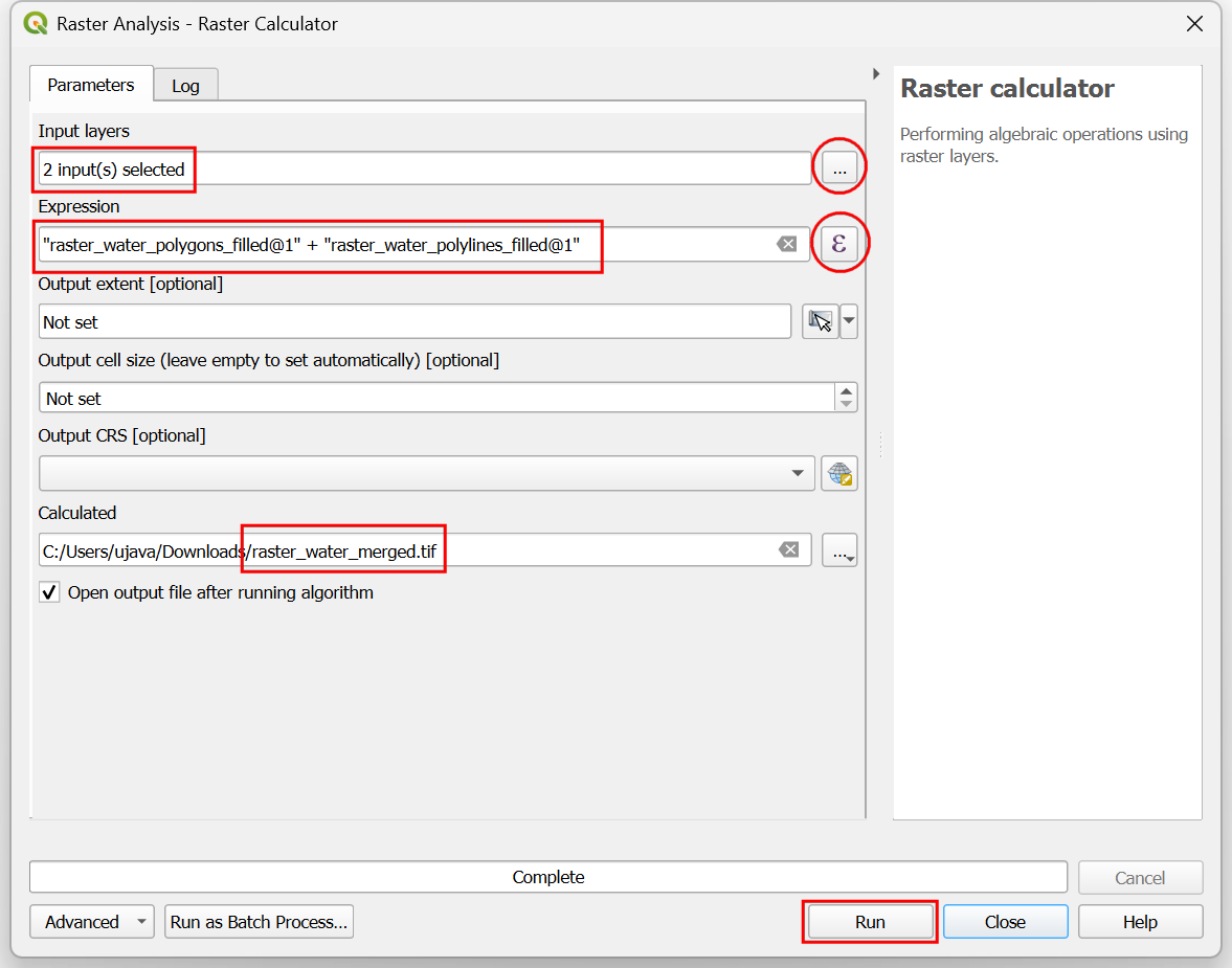

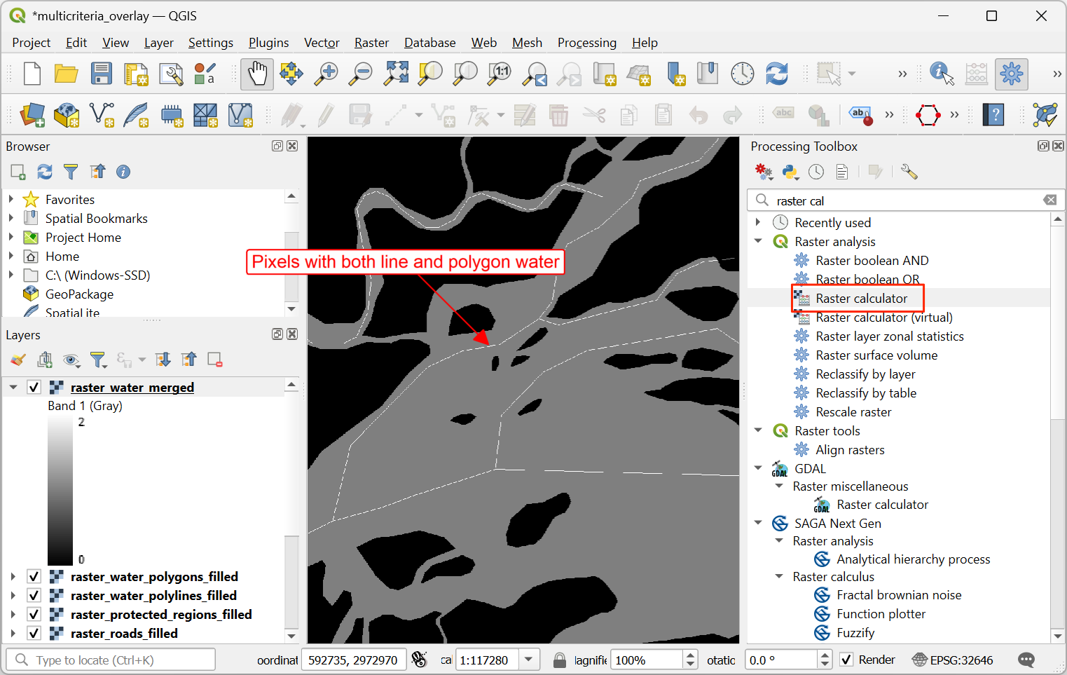
11. Het resulterende samengevoegde raster zal pixels hebben met de waarde 1 voor alle gebieden met water. Maar het zal u opvallen dat er sommige regio’s zijn waar zowel een waterpolygoon als een waterpolylijn was. Die gebieden zullen pixels hebben met de waarde 2 - wat niet juist is. We kunnen dit repareren met een eenvoudige expressie. Open het algoritme Rasteranalyse ‣ Rasterberekeningen opnieuw.

12. Selecteer de laag raster_water_merged met de knop … als Invoerlaag. Voer de volgende expressie in met de knop ε. Laat alle andere opties als standaard staan en sla de uitvoerlaag op met de naam raster_water_filled.tif en klik op Uitvoeren.

"raster_water_merged@1" > 0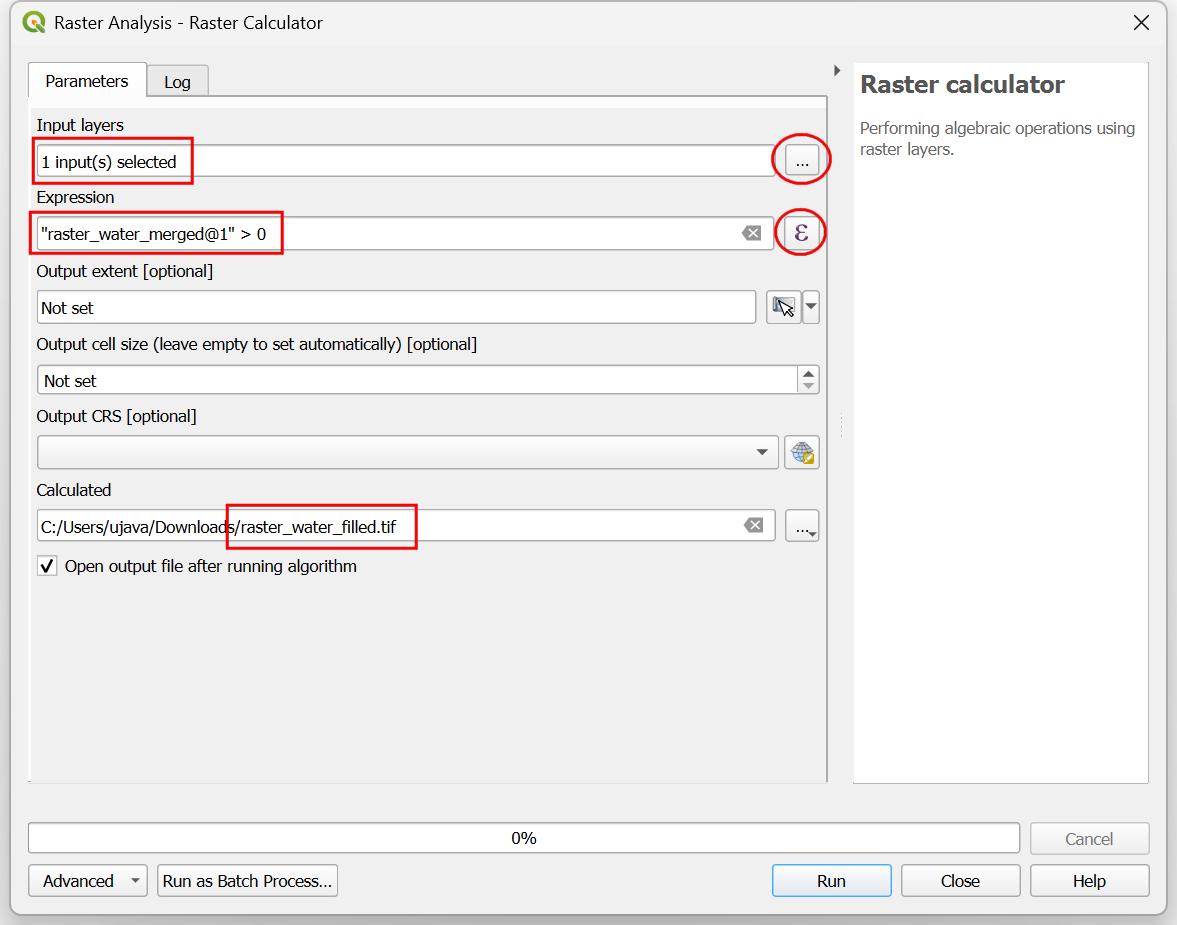

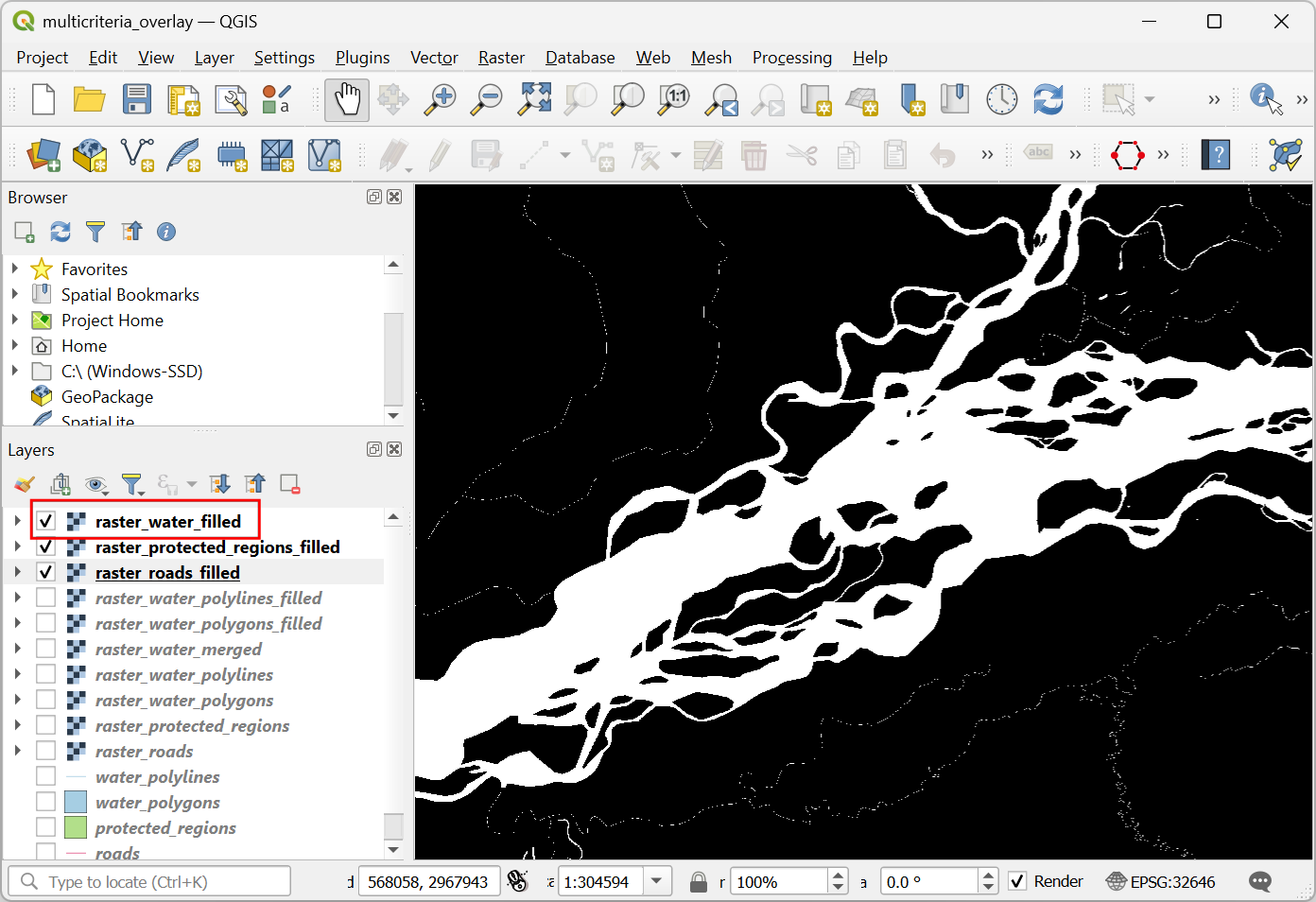
13. De resulterende laag raster_water_filled heeft nu pixels met alleen de waarden 0 en 1.

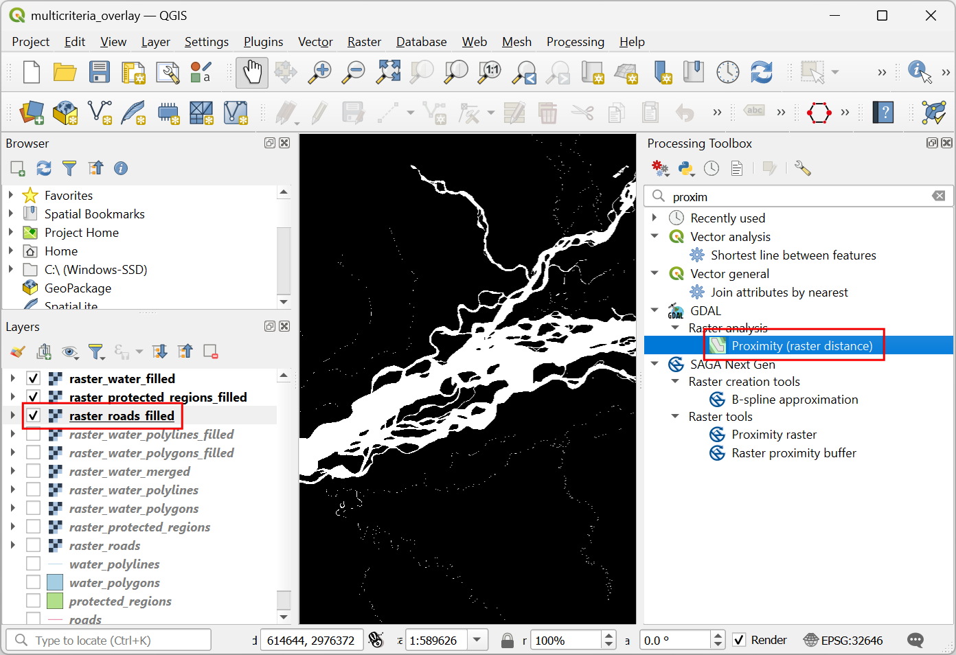
14. Nu we lagen hebben die pixels voor wegen en water weergeven, kunnen we rasters voor nabijheid maken. Deze zijn ook wel bekend als Euclidische afstanden - waar elke pixel in het uitvoerraster de afstand naar de dichtstbijzijnde pixel in de invoerlaag weergeeft. Dit resulterende raster kan dan worden gebruikt om geschikte gebieden te bepalen die binnen een bepaalde afstand vanaf de invoer liggen. Zoek naar en lokaliseer het algoritme GDAL ‣ Rasteranalyse ‣ Proximity (raster afstand). Dubbelklik er op om het te starten.

15. Selecteer, in het dialoogvenster Rasteranalyse -Proximity (raster afstand), raster_roads_filled als de Invoerlaag. Kies Coördinaten met geoverwijzingen als de Afstandseenheden. Omdat de invoerlagen in een geprojecteerd CRS staan met meters als de eenheden, voer 5000 (5 kilometer) in als de De maximale afstand die moet worden gegenereerd. Voor alle pixels, die verder weg liggen dan de maximale afstand, zullen we hun waarde ook op 5000 instellen. Stel dus de waarde voor Waarde Geen gegevens om te gebruiken voor het doel-nabijheidsraster in op 5000.

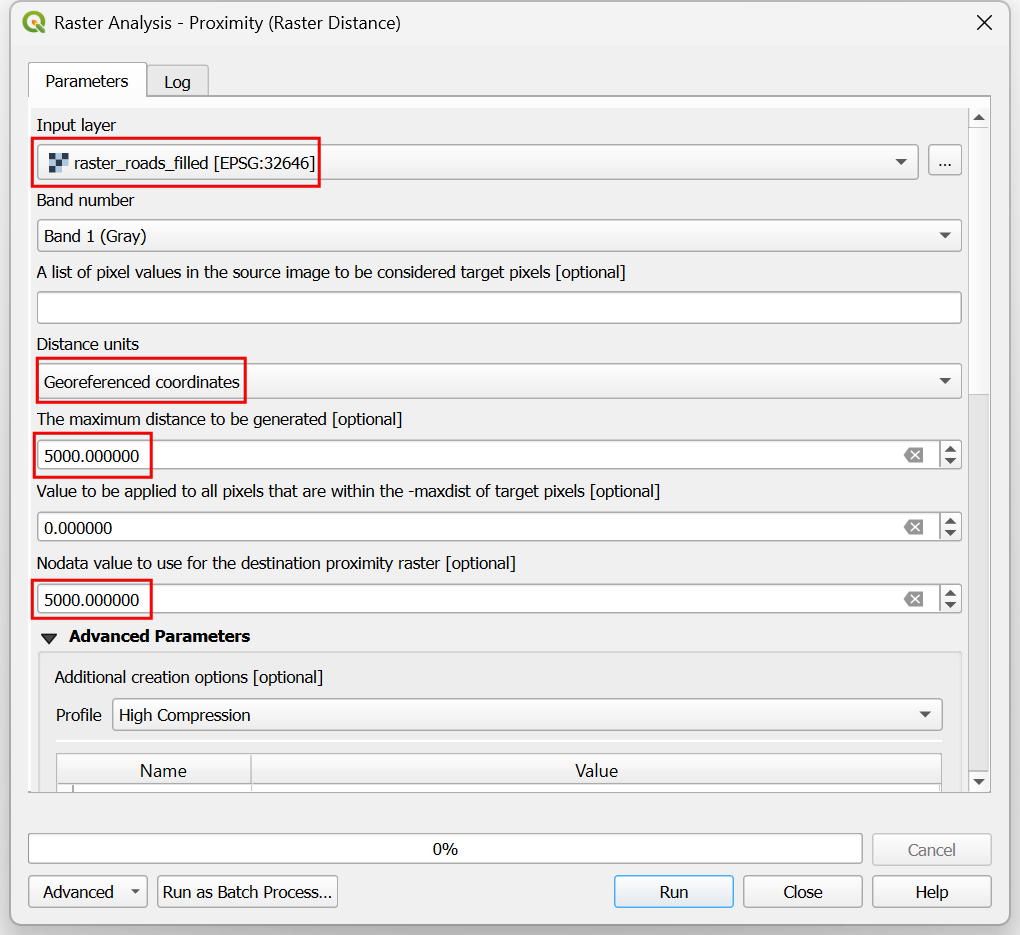
16. U kunt de Geavanceerde parameters vergroten en het profiel Hoge compressie selecteren om de compressie toe te passen. Noem het uitvoerbestand roads_proximity.tif en klik op Uitvoeren.

Notitie

Het kan ongeveer 15 minuten duren om dit proces uit te voeren. Het is een computertechnisch intensief algoritme dat de afstand moet berekenen voor elke pixel van het invoerraster.

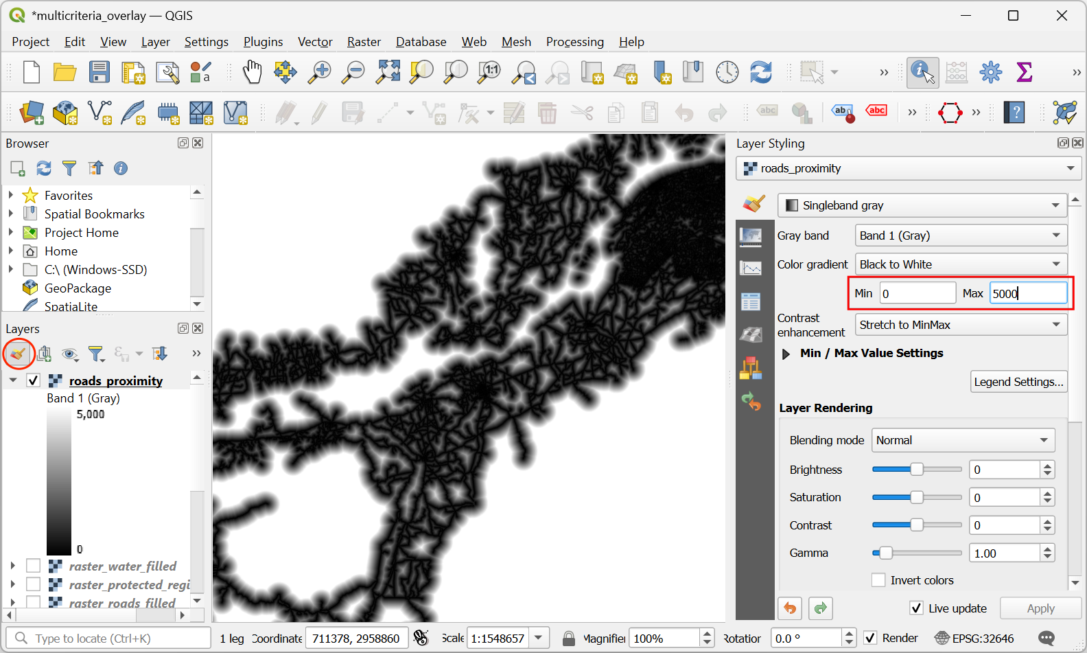
17. Als de verwerking is voltooid zal een nieuwe laag roads_proximity zijn toegevoegd aan het paneel Lagen. Laten we, om het beter te visualiseren, de standaard opmaak wijzigen. Klik op de knop Paneel Laag opmaken openen in het paneel Lagen. Wijzig de waarde Max onder Kleurovergang naar 5000.

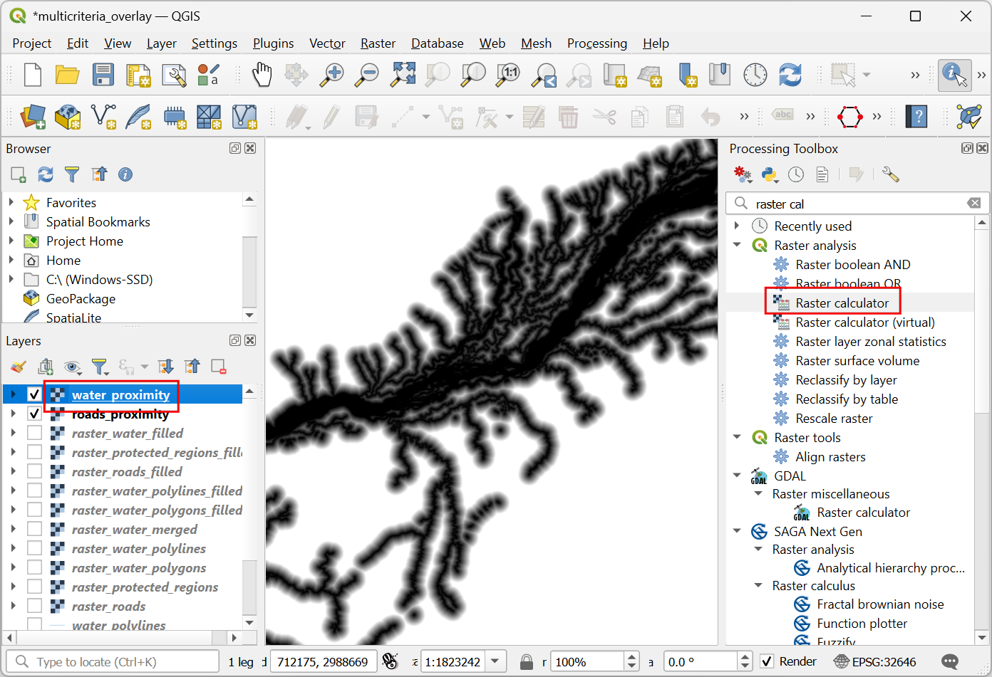
18. Herhaal het algoritme Proximity (raster afstand) voor de laag raster_water_filled met dezelfde parameters en noem de uitvoer water_proximity.tif. Als u willekeurig in het resulterende raster klikt, zult u zien dat het een continuüm is van waarden tussen 0 en 5000. We moeten, om dit raster te kunnen gebruiken in de overlay-analyse, het eerst opnieuw classificeren om afzonderlijke waarden te maken. Open het algoritme Rasteranalyse ‣ Rasterberekeningen opnieuw.

19. We willen een hogere score geven aan pixels die dichterbij wegen liggen. Dus laten we het volgens schema gebruiken.

• 0-1000m –> 100

• 1000-2000m –> 50

• >2000m –> 10

  Selecteer de laag roads_proximity met de knop … als Invoerlaag. Voer de volgende expressie in die de bovenstaande criteria toepast op de invoer. Laat alle andere opties als standaard staan en sla de uitvoerlaag op met de naam roads_reclass.tif en klik op Uitvoeren.

  100*("roads_proximity@1"<=1000)
      + 50*("roads_proximity@1">1000)*("roads_proximity@1"<=2000)
      + 10*("roads_proximity@1">2000)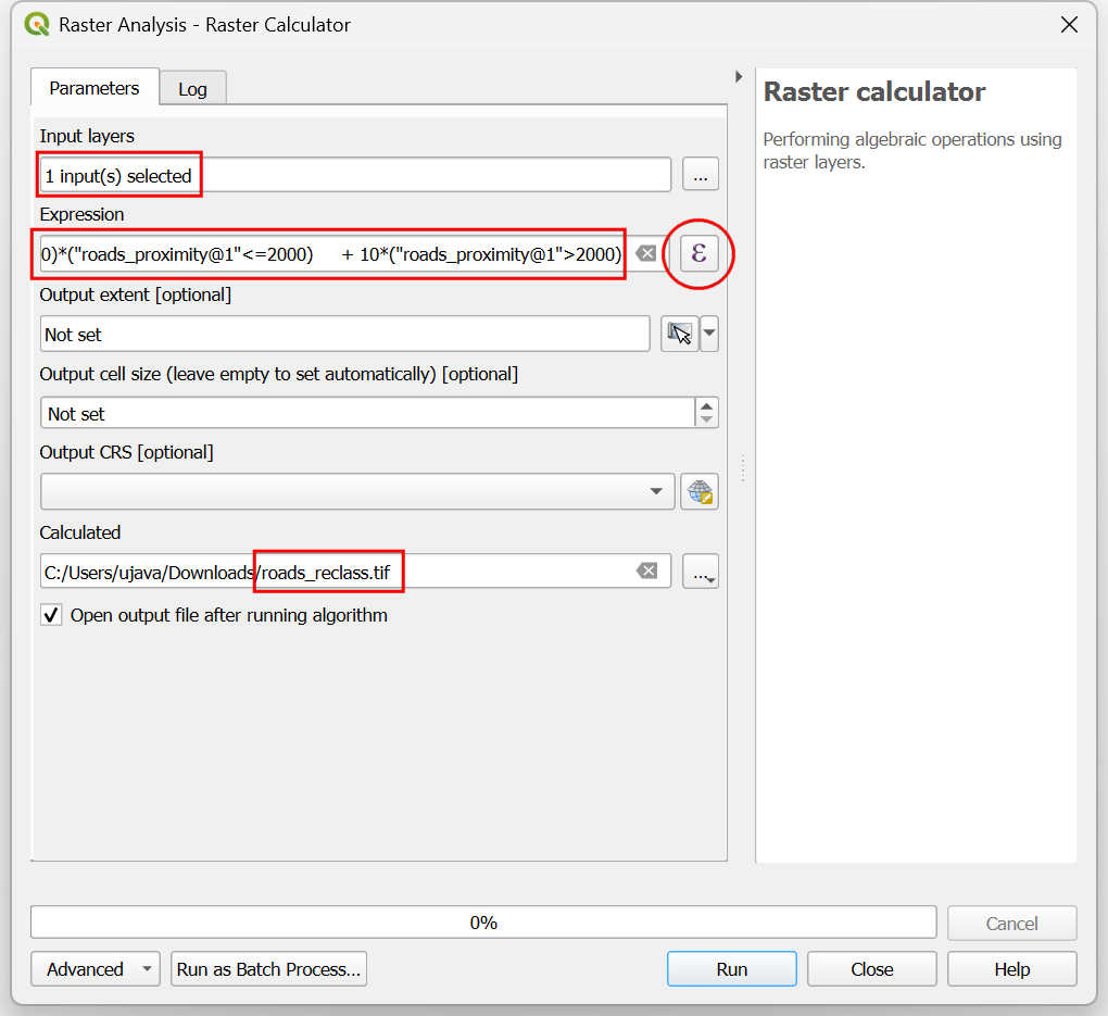
  

  

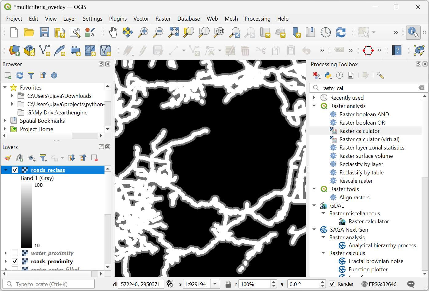
20. Als het proces voor opnieuw classificeren is voltooid, zal een nieuwe laag roads_reclass worden toegevoegd aan het paneel Lagen. Deze laag heeft slechts 3 verschillende waarden, 10, 50 en 100 die de relatieve geschiktheid van de pixels aangeven ten opzichte van de afstand vanaf wegen. Open het algoritme Rasteranalyse ‣ Rasterberekeningen opnieuw.

21. Herhaal het proces voor opnieuw classificeren voor de laag water_proximity. Hier zal het schema zijn omgedraaid, waarbij pixels die verder van water af liggen een hogere score zullen hebben.

• 0-1000m –> 10

• 1000 -2000m —> 50

• >2000m –> 100

  Selecteer de laag water_proximity met de knop … als Invoerlaag. Voer de volgende expressie in die de bovenstaande criteria toepast op de invoer. Laat alle andere opties als standaard staan en sla de uitvoerlaag op met de naam water_reclass.tif en klik op Uitvoeren.

  100*("water_proximity@1">2000)
  + 50*("water_proximity@1">1000)*("water_proximity@1"<=2000)
  + 10*("water_proximity@1"<1000)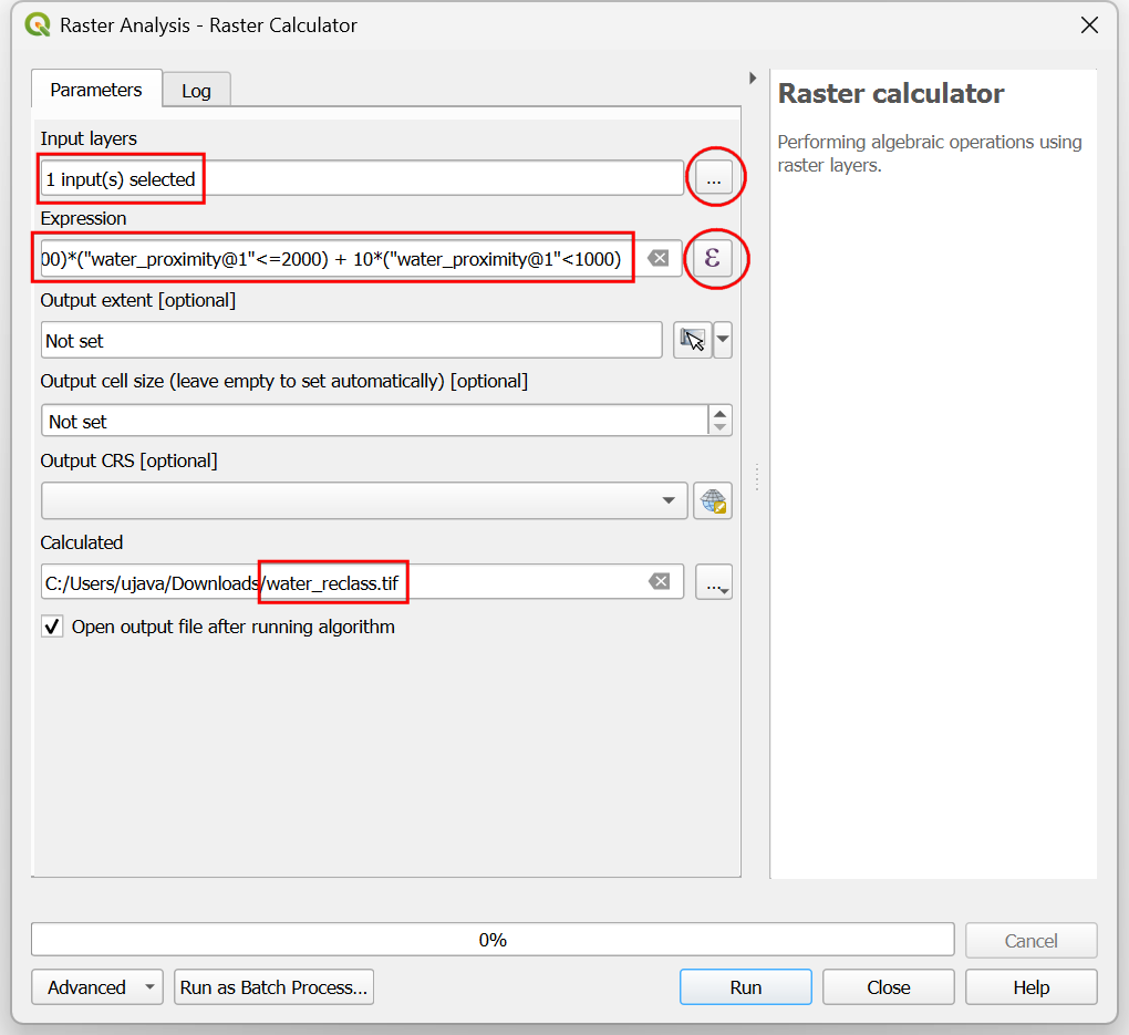
  

  

22. Nu zijn we klaar om de uiteindelijke overlay-analyse uit te voeren. Weet nog dat onze criteria voor het bepalen van de geschiktheid de volgende waren - dicht bij wegen, weg van het water en niet in een beschermde regio. Open Rasteranalyse ‣ Rasterberekeningen. Selecteer de lagen roads_reclass, water_reclass, raster_protected_regions_filled met de knop … als Invoerlagen. Gebruik de knop ε om de volgende expressie in te voeren die deze criteria toepast. Laat alle andere opties als standaard staan. Noem de uitvoer overlay.tif en klik op Uitvoeren.

(("roads_reclass@1" + "water_reclass@1")/2)
*("raster_protected_regions_filled@1"  !=  1 )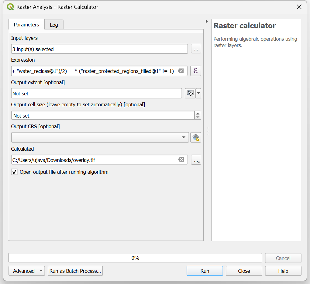

Notitie

In dit voorbeeld geven we een gelijk gewicht aan zowel de nabijheid van wegen als van water. In een scenario voor de echte wereld zou u meerdere criteria met een verschillende mate van belangrijkheid kunnen hebben. U kunt dat simuleren door de rasters met het toepasselijke gewicht in de bovenstaande expressie te vermenigvuldigen. Bijvoorbeeld als nabijheid van wegen twee keer zo belangrijk is als nabijheid van water, zou u, in plaats van (("roads_reclass@1" + "water_reclass@1")/2), de expressie ((2*"roads_reclass@1" + "water_reclass@1")/3) kunnen gebruiken.

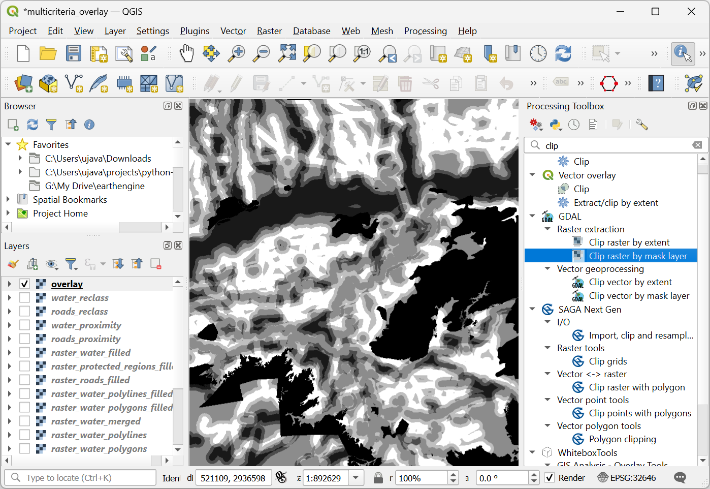
23. Als de verwerking is voltooid, zal de resulterende raster overlay worden toegevoegd aan het paneel Lagen. De pixelwaarden in dit raster liggen tussen 0 en 100 - waar 0 het minst geschikte en 100 het meest geschikte gebied voor ontwikkeling is. Laten we de resultaten bijknippen tot de laag boundary. Open het algoritme Raster uitnemen ‣ Raster op maskerlaag clippen.

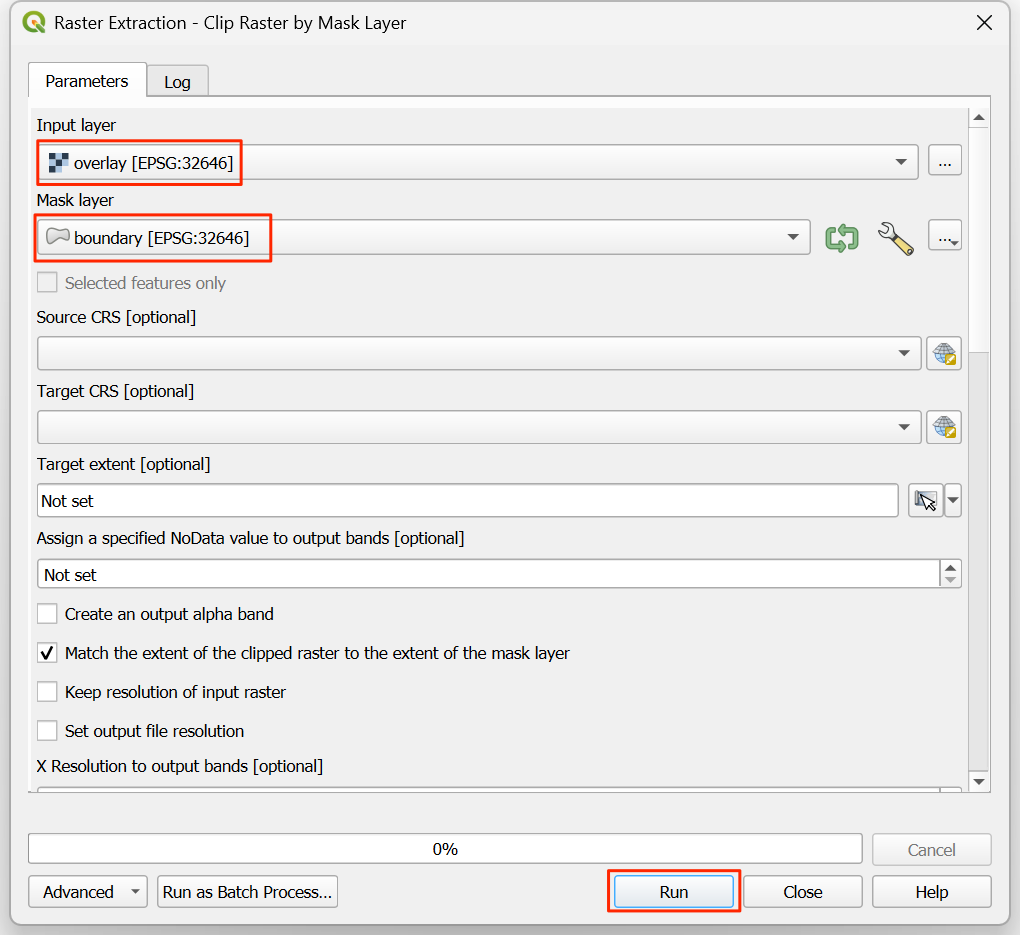
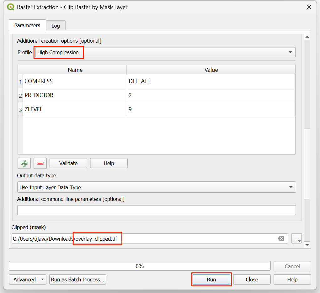
24. In het dialoogvenster Raster uitnemen - Raster op maskerlaag clippen, selecteer overlay als de Invoerlaag en boundary als de Maskeerlaag.

25. Scroll naar beneden naar de Geavanceerde parameters en selecteer het profiel Hoge compressie selecteren om de compressie toe te passen. Benoem de laag Geclipt (masker) als roads_proximity.tif en klik op Uitvoeren.

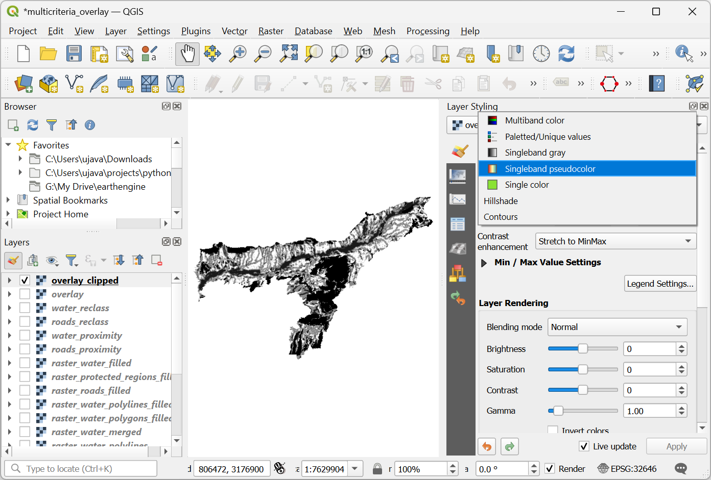
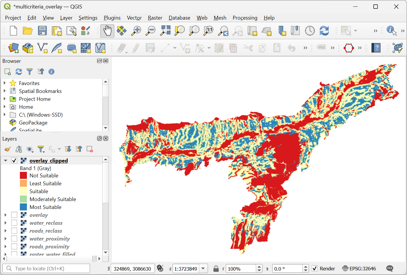
26. Als de verwerking eenmaal is voltooid zal de uiteindelijke uitvoerlaag overlay_clipped worden toegevoegd aan het paneel Lagen. Klik op de knop Paneel Laag opmaken openen in het paneel Lagen en selecteer de renderer Enkelband pseudokleur.

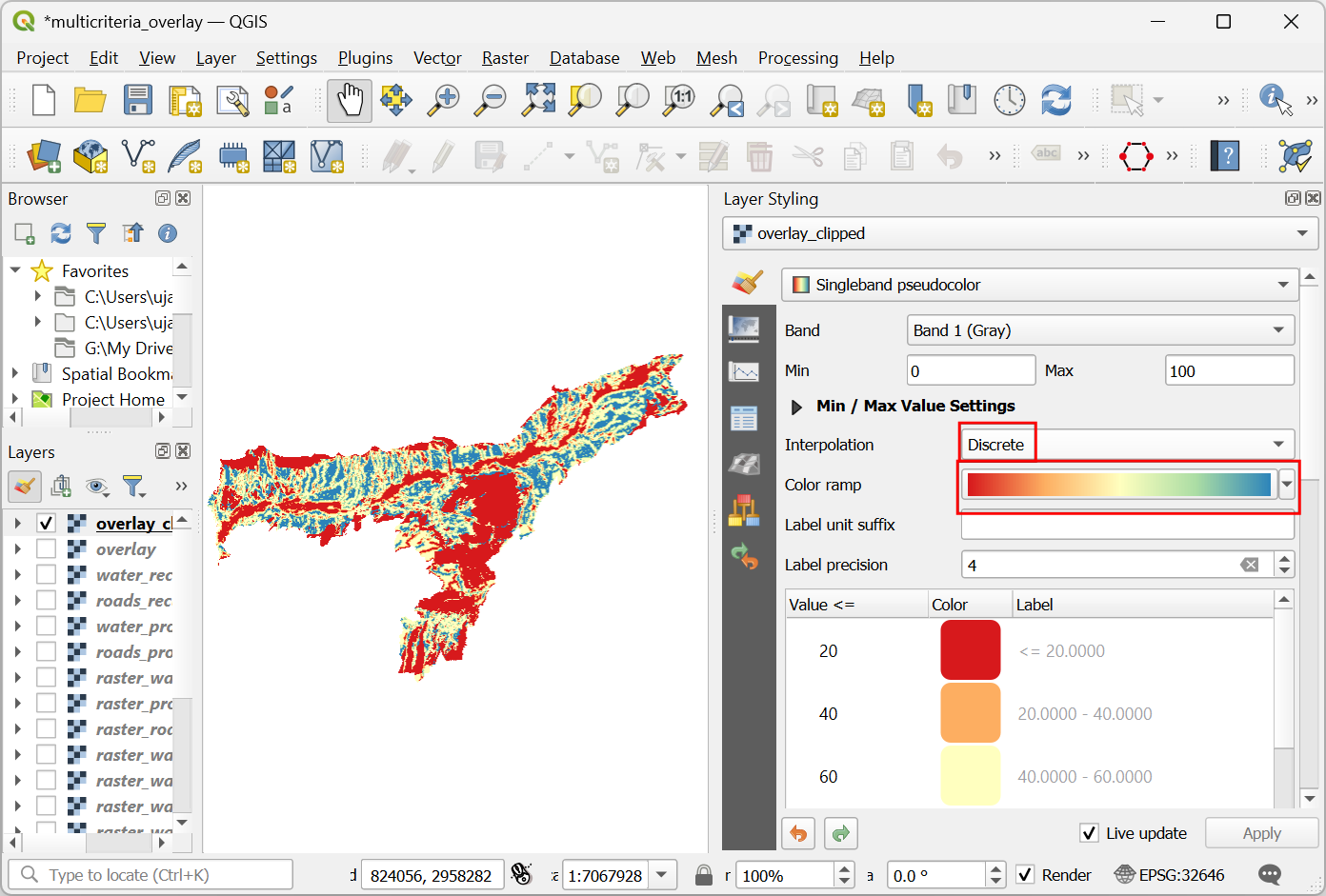
27. Stel de Interpolatie in op Afzonderlijk en kies het kleurverloop Spectral.

28. Klik op de standaard labelwaarden naast elke kleur en voer toepasselijke labels in.

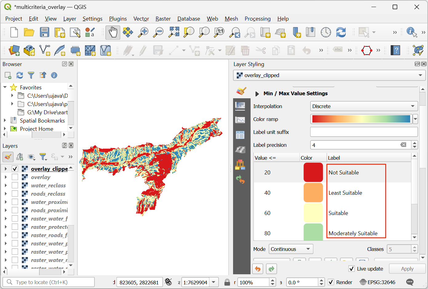
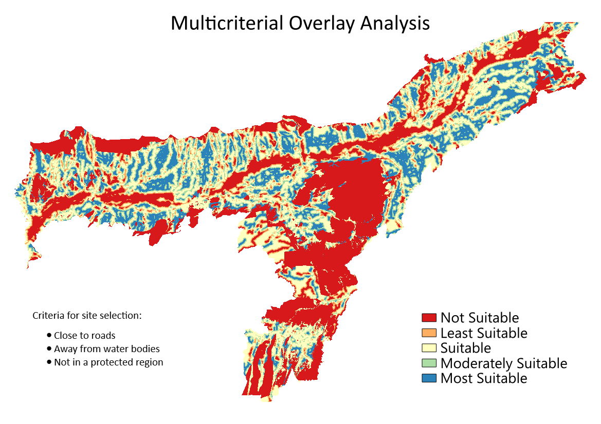
29. De labels zullen ook als Legenda verschijnen onder de laag overlay_clipped. Dit is onze uiteindelijke kaart die de geschiktheid van de plaatsen aangeeft, overeenkomstig de gekozen criteria.

---

If you want to give feedback or share your experience with this tutorial, please comment below. (requires GitHub account)