Analiza prekrivanja po več kriterijih (QGIS3)

Večkriterijska ponderirana analiza je postopek dodeljevanja območij na podlagi različnih lastnosti, ki jih morajo imeti izbrana območja. Čeprav je to običajna operacija GIS, jo je najbolje izvesti v rastrskem prostoru z uporabo pristopa, ki temelji na mreži.

Opomba

Vektorsko in rastrsko prekrivanje

You can do the overlay analysis on vector layers using geoprocessing tools such as buffer, dissolve, difference and intersection. This method is ideal if you wanted to find a binary suitable/non-suitable answer and you are working with a handful of layers. You can review our video tutorial on Locating A New Bicycle Parking Station using Multicriteria Overlay Analysis for a step-by-step guide on this approach.

Delo v rastrskem prostoru vam omogoča razvrstitev primernosti - ne le najprimernejše lokacije. Omogoča tudi enostavno združevanje poljubnega števila vhodnih slojev in dodeljevanje različnih uteži posameznim merilom. Na splošno je to najprimernejši pristop za ugotavljanje primernosti lokacije.

V tem učbeniku je predstavljen tipičen potek dela za izvedbo analize primernosti lokacije - pretvorba izvornih vektorskih podatkov v ustrezne rastre, njihova ponovna razvrstitev in izvajanje matematičnih operacij.

Pregled naloge

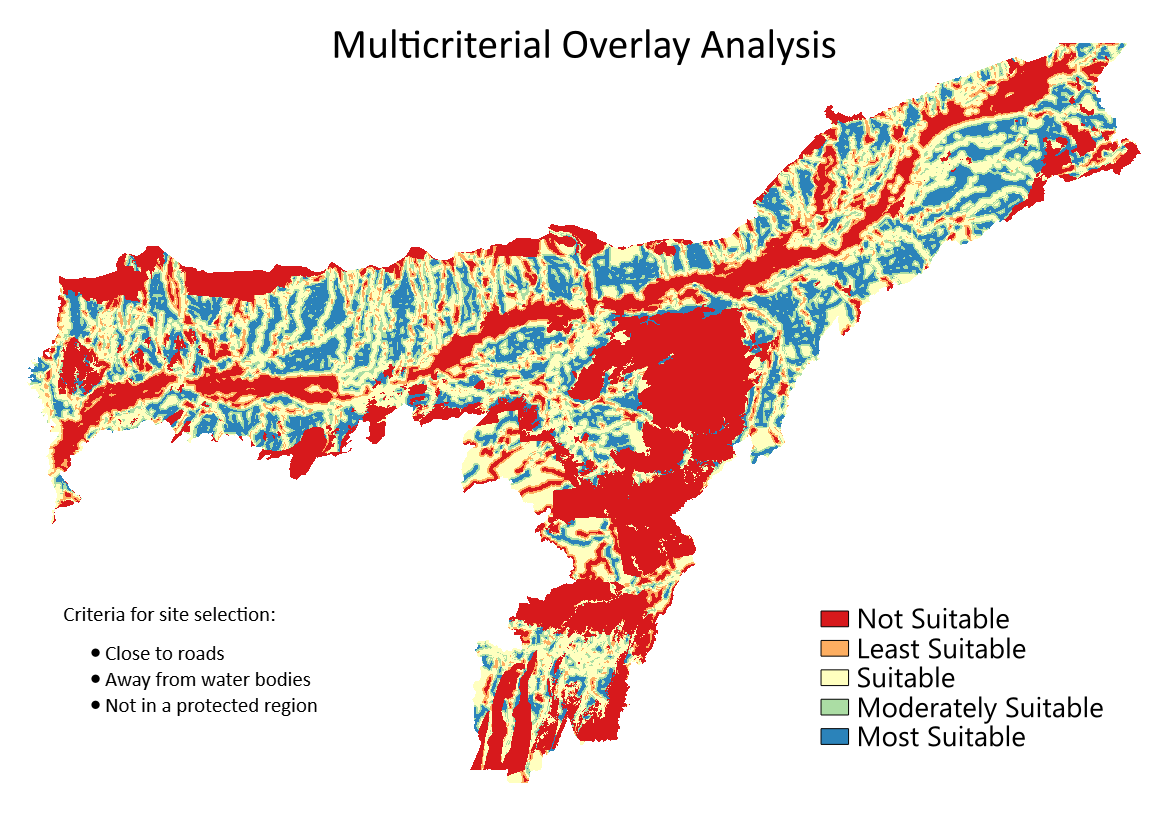
V tem učbeniku bomo opredelili primerna področja za razvoj, in sicer

• Blizu cest in

• Stran od vodnih teles in

• Ne na zaščitenem območju.

Pridobivanje podatkov

Uporabili bomo vektorske podatkovne sloje iz OpenStreetMap (OSM). OSM je globalna podatkovna zbirka prosto dostopnih osnovnih kartografskih podatkov. Geofabrik zagotavlja dnevno posodobljene shapefile podatkovnih nizov OpenStreetMap.

We will be using the OSM data layers for the state of Assam in India. Geofabrik India shapefiles were downloaded, reprojected to a UTM projection, clipped to the state boundary and packaged in a single GeoPackage file. You can download a copy of the geopackage from the link below:

assam.gpkg

Vir podatkov: [GEOFABRIK]

Postopek

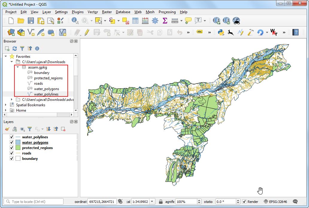
1. V brskalniku QGIS poiščite preneseno datoteko assam.gpkg. Razširite jo in povlecite vsakega od petih posameznih podatkovnih slojev na platno zemljevida. Na plošči Layers boste videli naložene sloje boundary, roads, protected_regions, water_polygons in water_polylines.

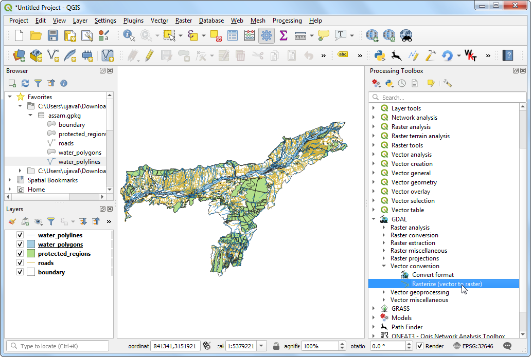
2. First step in the overlay analysis, is to convert each data layer to raster. An important consideration is that all rasters must be of the same extent. We will use the boundary layer as the extent for all the rasters. Go to Processing ‣ Toolbox. Search for and locate the GDAL ‣ Vector conversion ‣ Rasterize (vector to raster) algorithm. Double-click to launch it.

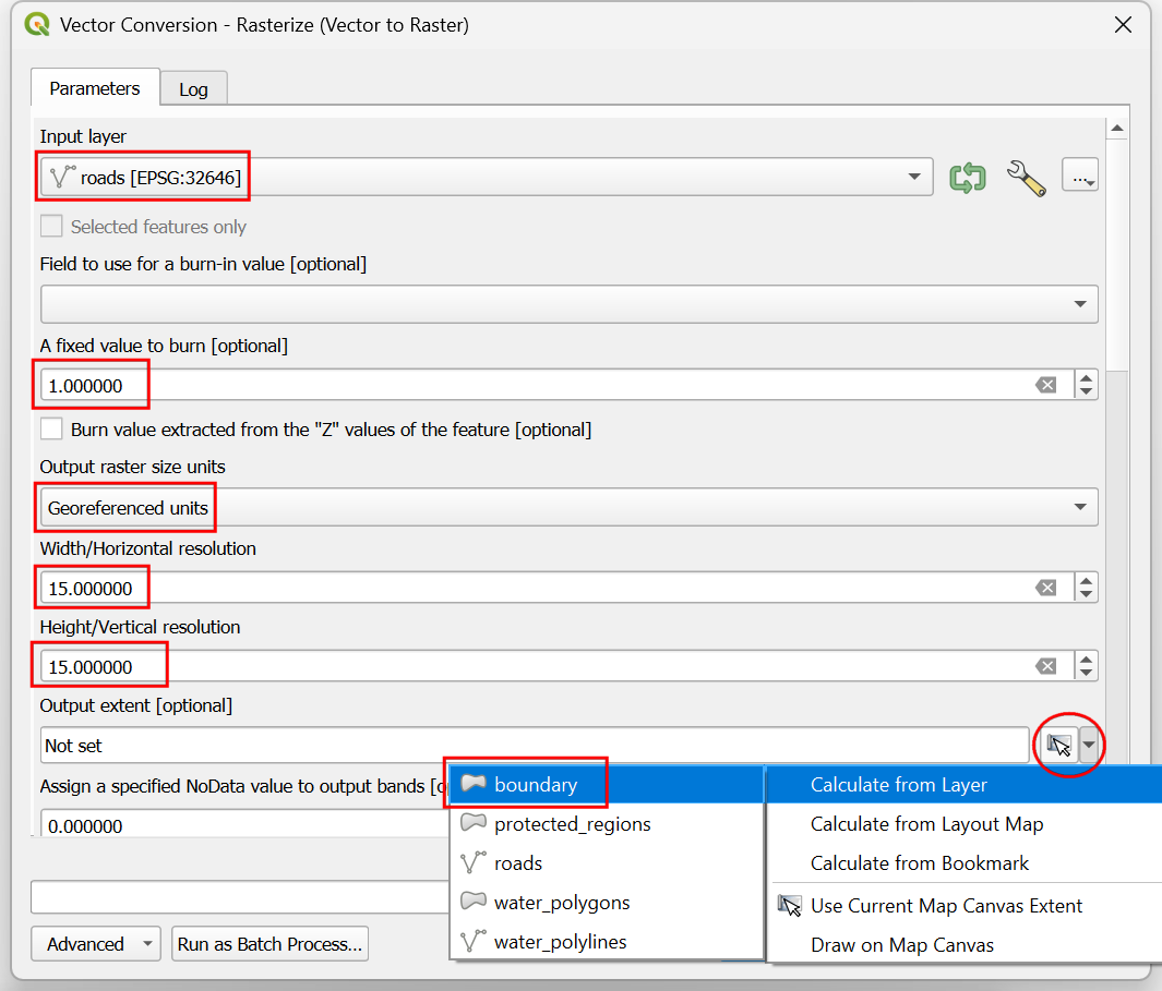
3. In the Vector Conversion - Rasterize (vector to raster) dialog, select roads as the Input layer. We want to create an output raster where pixel values are 1 where there is a road and 0 where there are no roads. Enter 1 as the A fixed value to burn. The input layers are in a projected CRS with meters are the unit. Select Geoferenced units as the Output raster size units. We will set the resolution of the output raster to be 15 meters. Select 15 as both Width/Horizontal resolution and Height/Vertical resolution. Next, click the arrow next to Output extent and select Calculate from Layer ‣ boundary.

4. Scroll down to find the Advanced Parameters and select the profile High Compression to apply the compression. This will generate the compressed raster file of smaller size after running the tool. Applying lossless compression is highly recommended while working with raster data.

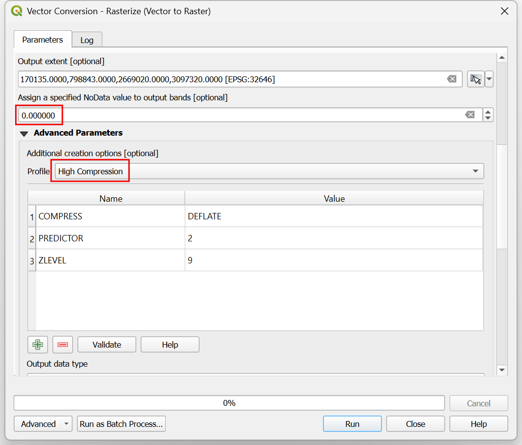
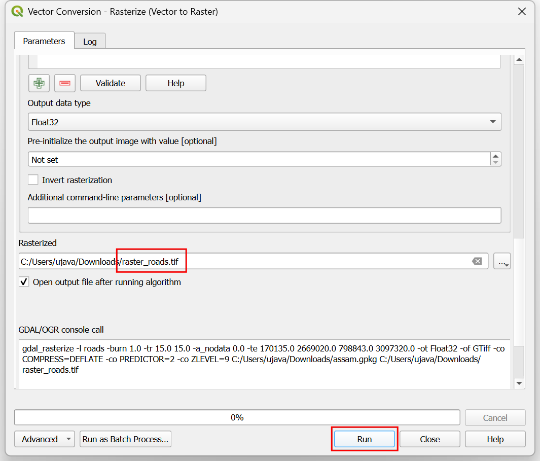
5. Set the Rasterized output raster as raster_roads.tif and click Run.

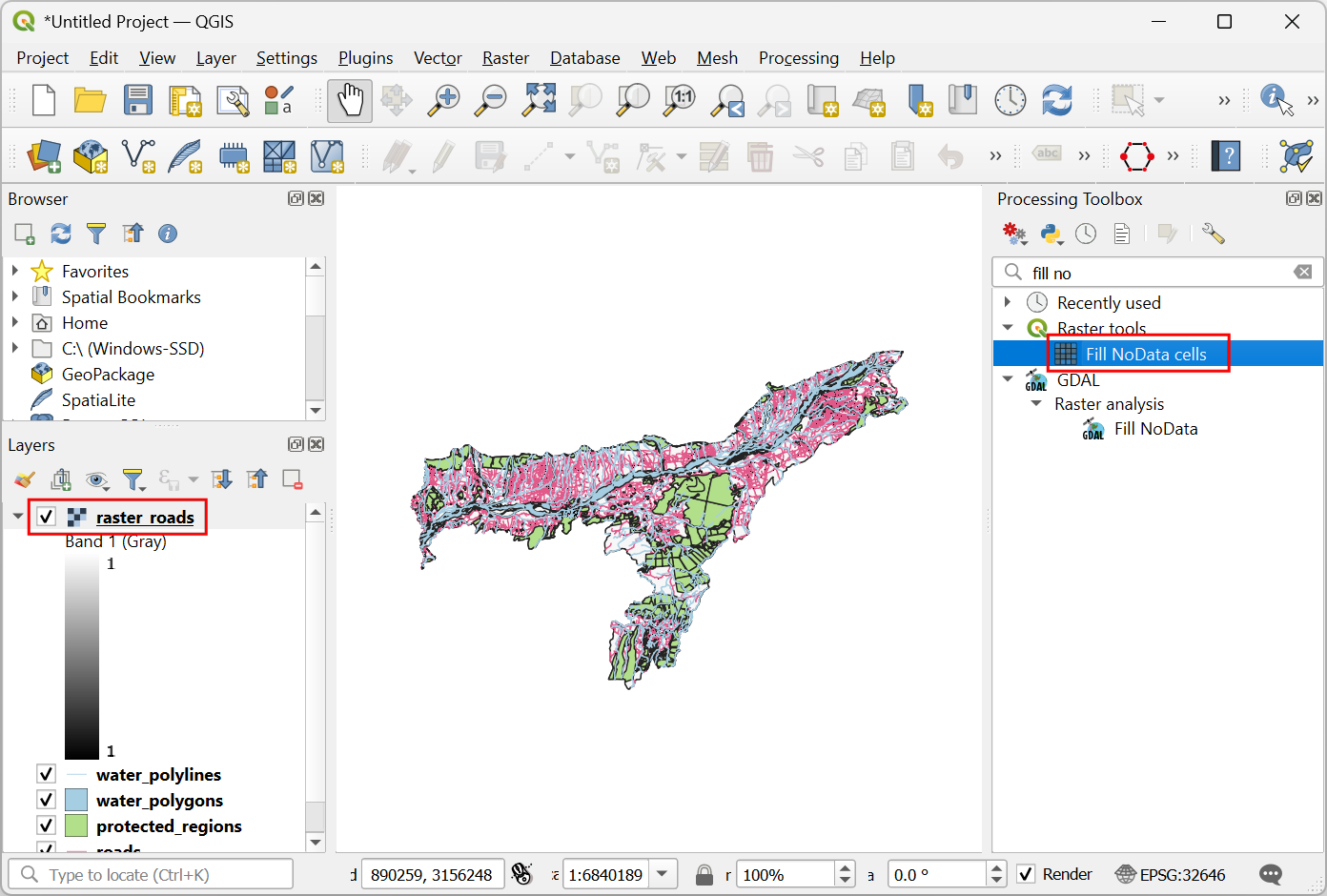
6. Once the processing finishes, you will see a new layer raster_roads loaded in the Layers panel. The raster has pixel values 1 for pixels which intersected with the roads. All other pixels are set as NoData values. These nodata values are problematic because when raster calculator (which we will use later) encounters a pixel with nodata value in any layer, it sets the output value of that pixel to nodata as well, resulting is unexpected output. We will fill these nodata values with the value 0. Search for and locate the Raster Tools ‣ Fill NoData cells algorithm. Double-click to launch it.

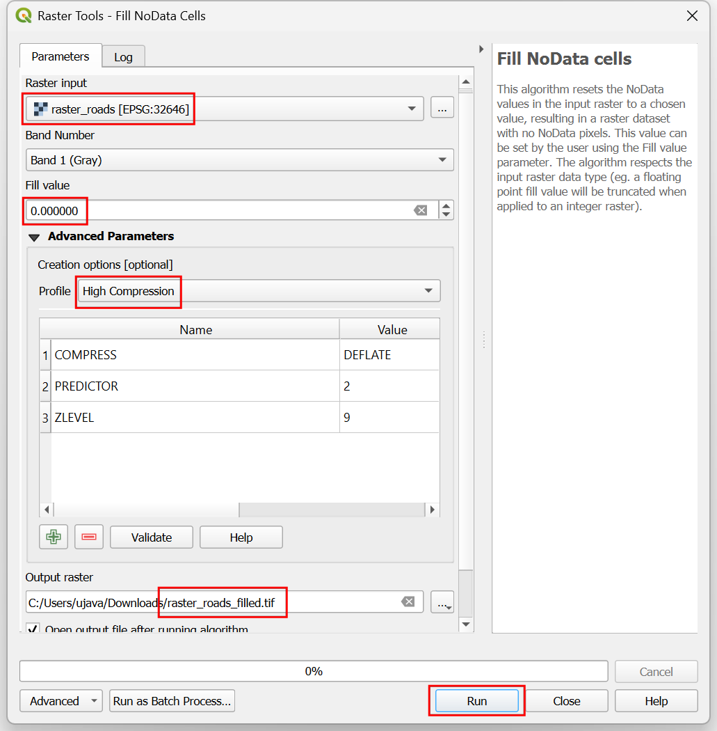
7. Select raster_roads as the Raster input and choose 0 as the Fill value. Scroll down to find the Advanced Parameters and select the profile High Compression to apply the compression. Set the Output raster as raster_roads_filled.tif and click Run.

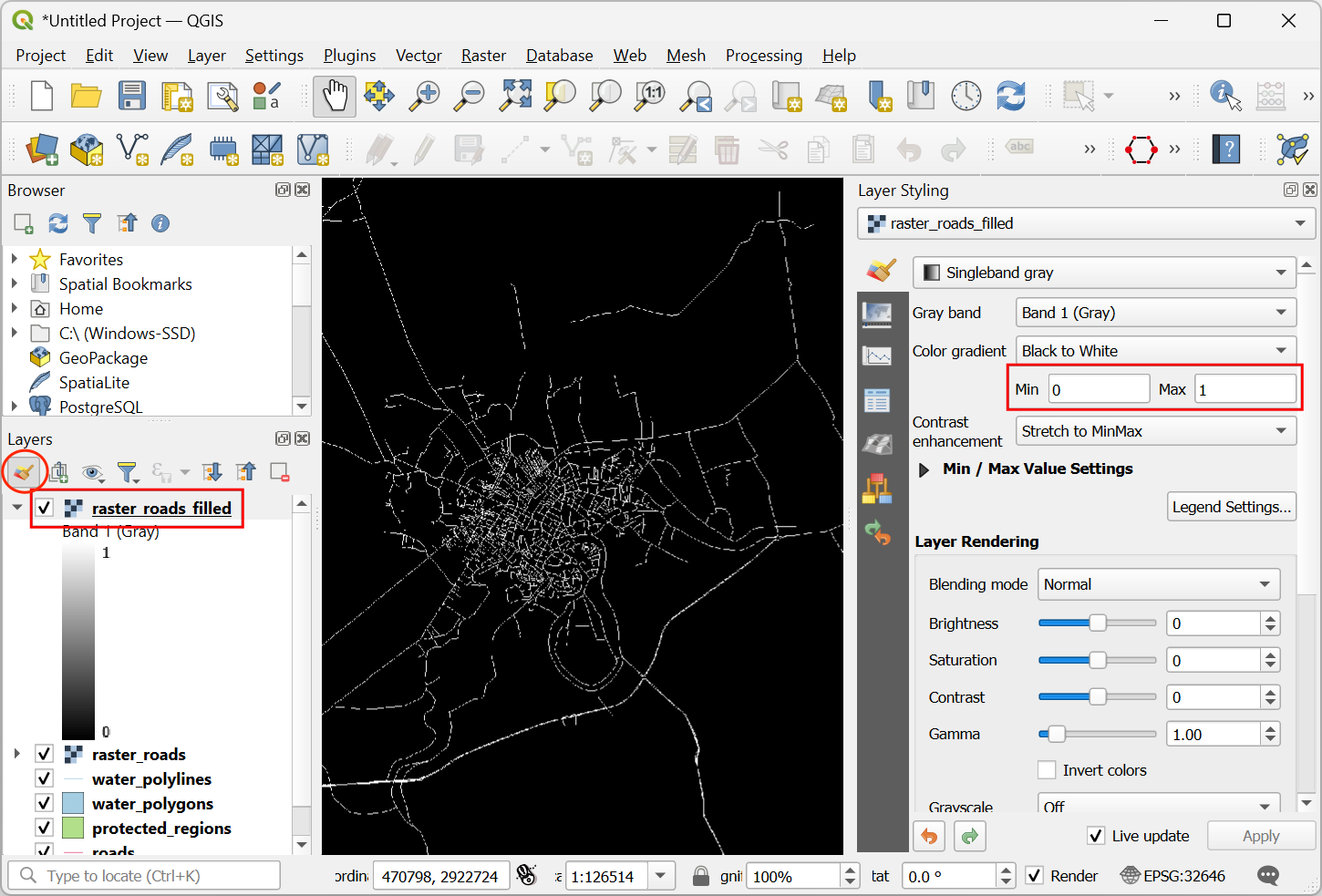
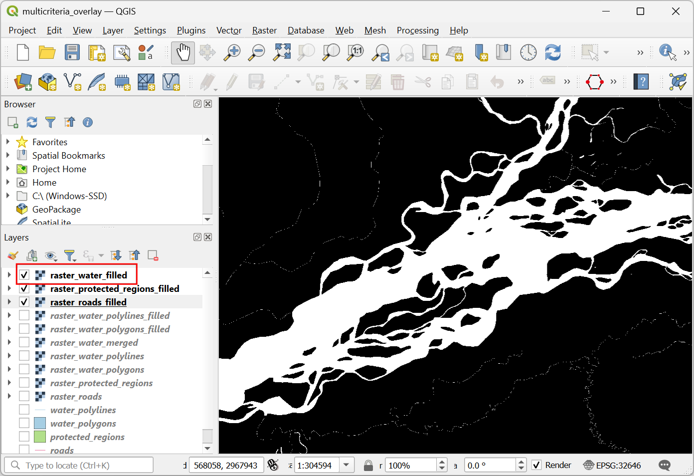
8. Once the processing finishes, you will see the new layer raster_roads_filled loaded in the Layers panel. This raster has values 1 for roads and 0 for no roads. If the layer is not visualized correctly, you can click the Open the Layer Styling Panel and set the Min to 0 and Max to 1.

9. Repeat steps 3-8 for the other 3 vector layers protected_regions, water_polylines and water_polygons layers. You need to rasterize and fill the nodata cells for these layers. If you want to run these steps manually, you can configure the processing algorithm dialog, run the algorithm and once the algorithm finishes, switch to the Parameters tab and just change the input and output layer names. You can also run each algorithm on all 4 layers in a single step using Batch Processing. See the Batch Processing using Processing Framework (QGIS3) tutorial to learn more. Once you are done, you should have 4 raster layers and generate the corresponding raster layers raster_roads_filled, raster_protected_regions_filled, raster_water_polylines_filled and raster_water_polygons_filled. You will notice that we have 2 water related layers - both representing water. We can merge them to have a single layer representing water areas in the region. Search for and locate Raster analysis ‣ Raster calculator algorithm in the Processing Toolbox. Double-click to launch it.

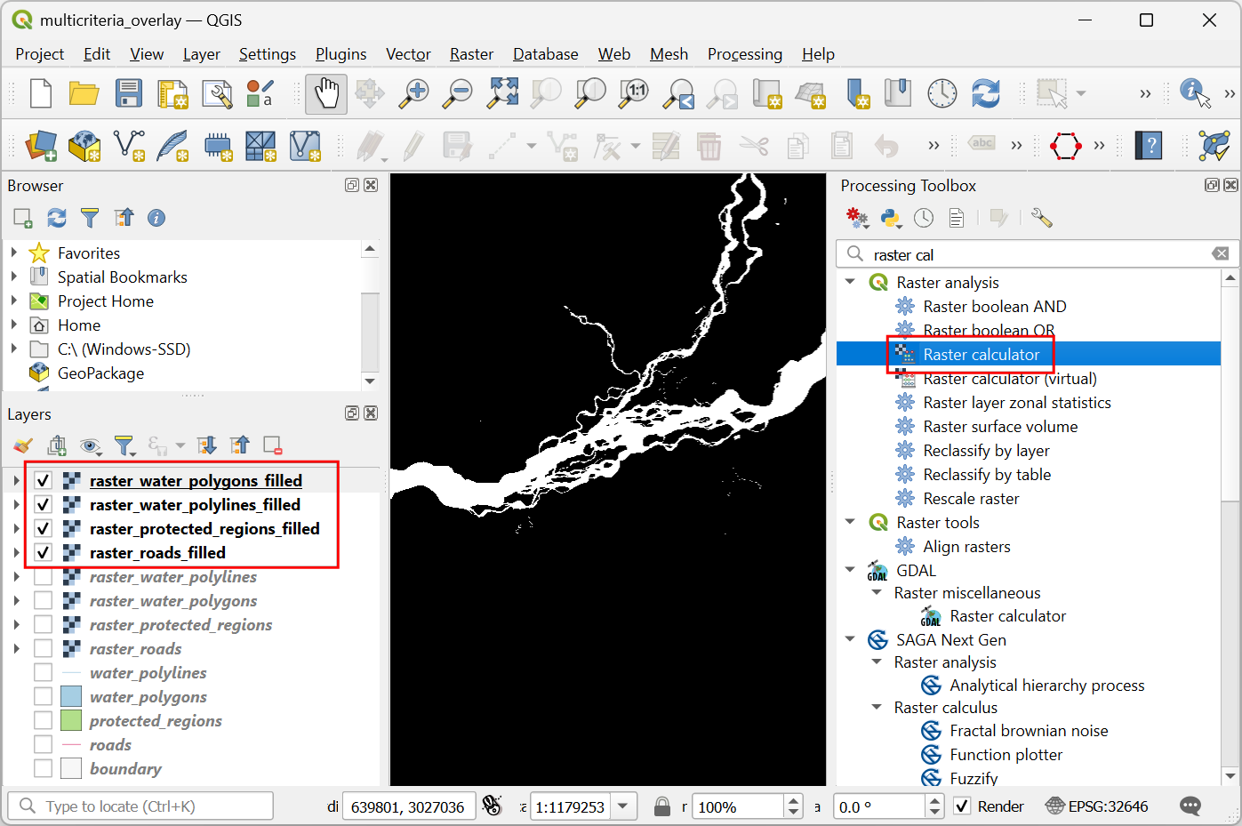
10. Select raster_water_polygons and raster_water_polylines layers using … button as Input Layers. Enter the following expression using ε button. Keep all the other options as default and save the output layer with the name raster_water_merged.tif and click Run.

"raster_water_polygons_filled@1" + "raster_water_polylines_filled@1"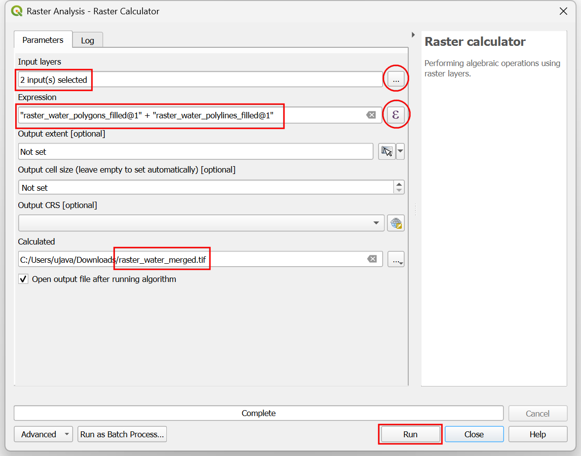

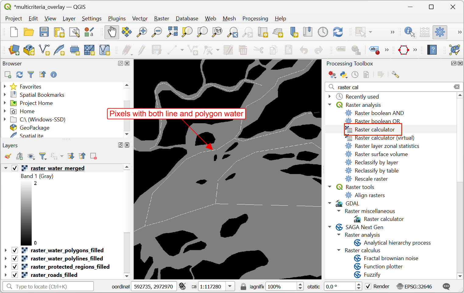
11. Tako združen raster bo imel piksle z vrednostjo 1 za vsa območja z vodo. Opazili pa boste, da je na nekaterih območjih obstajal tako poligon z vodo kot poligon z vodo. Ta območja bodo imela piksle z vrednostjo 2, kar ni pravilno. To lahko popravimo s preprostim izrazom. Ponovno odprite algoritem Raster analysis ‣ Raster calculator.

12. Select raster_water_merged layer using … button as an Input Layer. Enter the following expression using ε button. Keep all the other options as default and save the output layer with the name raster_water_filled.tif and click Run.

"raster_water_merged@1" > 0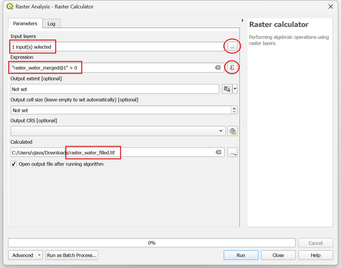

13. The resulting layer raster_water_filled now has pixels with only 0 and 1 values.

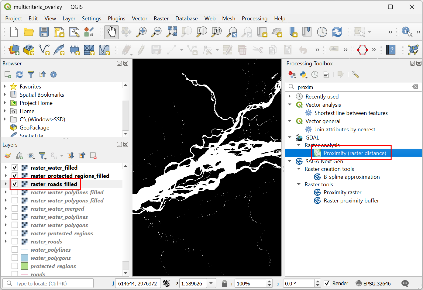
14. Zdaj, ko imamo plasti, ki predstavljajo piksle cest in vode, lahko ustvarimo rastre bližine. Ti so znani tudi kot evklidske razdalje - vsaka piksla v izhodnem rastru predstavlja razdaljo do najbližjega piksla v vhodnem rastru. Ta dobljeni raster lahko nato uporabimo za določitev primernih območij, ki so v določeni razdalji od vhodnega. Poiščite in najdite algoritem GDAL ‣ Raster analysis ‣ Proximity (raster distance). Z dvojnim klikom ga zaženite.

15. In the Raster Analysis - Proximity (Raster Distance) dialog, select raster_roads_filled as the Input layer. Choose Georeferenced coordinates as the Distance units. As the input layers are in a projected CRS with meters as the units, enter 5000 (5 kilometers) as the Maximum distance to be generated. For all pixels that are more than the maximum distance away - we will set their values to be 5000 as well. So set the Nodata value to use for the destination proximity raster value to 5000.

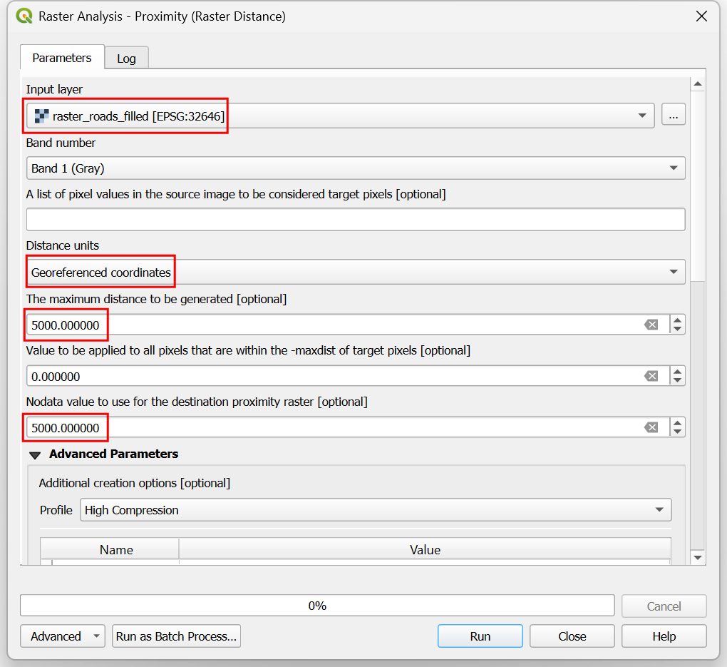
16. You can expand the Advanced Parameters and select the profile High Compression to apply the compression. Name the output file as roads_proximity.tif and click Run.

Opomba

It may take upto 15 minutes for this process to run. It is a computationally intensive algorithm that needs to compute distance for each pixel of the input raster.

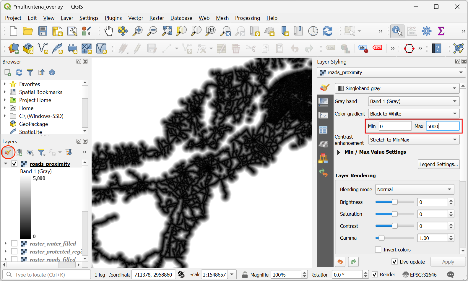
17. Po končani obdelavi bo na ploščo Layers dodan nov sloj roads_proximity. Za boljšo vizualizacijo spremenimo privzeto oblikovanje. Kliknite gumb Open the Layer Styling panel na plošči Layers. Vrednost Max spremenite na 5000 v razdelku Color gradient.

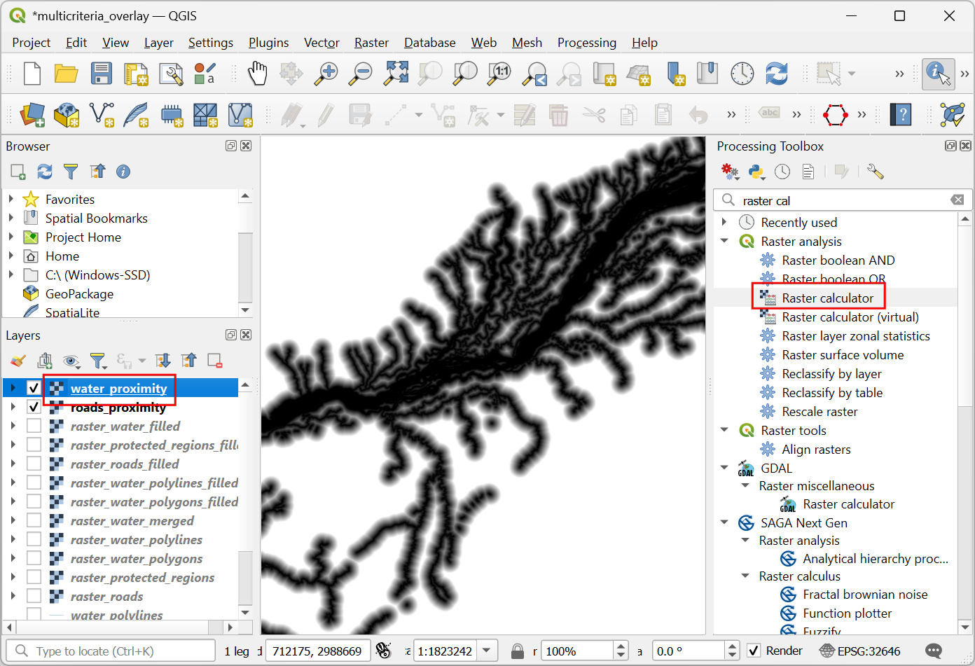
18. Repeat the Proximity (Raster Distance) algorithm for the raster_water_filled layer with same parameters and name the output water_proximity.tif. If you click around the resulting raster, you will see that it is a continuum of values from 0 to 5000. To use this raster in overlay analysis ,we must first re-classify it to create discrete values. Open Raster analysis ‣ Raster calculator algorithm again.

19. Pikslom, ki so v bližini cest, želimo dodeliti višje število točk. Zato uporabimo naslednjo shemo.

• 0-1000m -> 100

• 1000-2000m –> 50

• >2000m –> 10

  Select roads_proximity layer using … button as an Input Layer. Enter the following expression that applies the above criteria on the input. Keep all the other options as default and save the output layer with the name roads_reclass.tif and click Run.

  100*("roads_proximity@1"<=1000)
      + 50*("roads_proximity@1">1000)*("roads_proximity@1"<=2000)
      + 10*("roads_proximity@1">2000)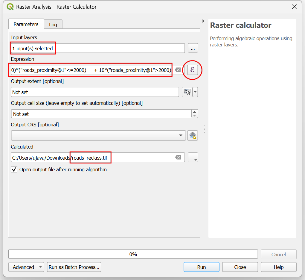
  

  

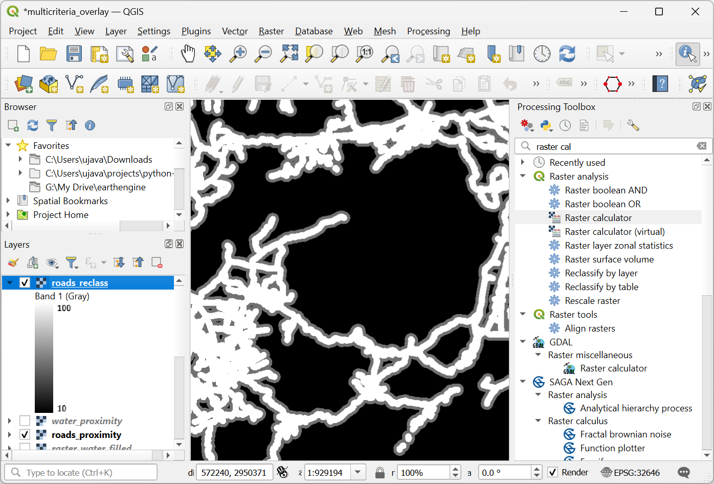
20. Ko se postopek preklasifikacije konča, se na ploščo Layers doda nov sloj roads_reclass. Ta sloj ima samo tri različne vrednosti, 10, 50 in 100, ki označujejo relativno primernost pikslov glede na oddaljenost od cest. Ponovno odprite algoritem Raster analysis ‣ Raster calculator.

21. Ponovite postopek ponovnega razvrščanja za sloj water_proximity. Tu bo shema obratna, saj bodo piksli, ki so bolj oddaljeni od vode, imeli višje število točk.

• 0-1000m -> 10

• 1000 -2000m —> 50

• >2000m –> 100

  Select water_proximity layer using … button as an Input Layer. Enter the following expression hat applies the above criteria on the input. Keep all the other options as default and save the output layer with the name water_reclass.tif and click Run.

  100*("water_proximity@1">2000)
  + 50*("water_proximity@1">1000)*("water_proximity@1"<=2000)
  + 10*("water_proximity@1"<1000)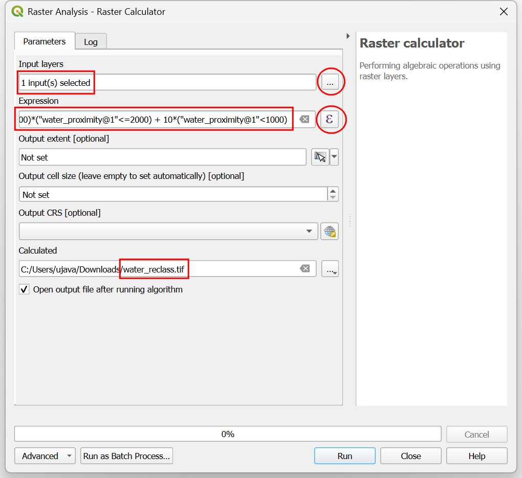
  

  

22. Now we are ready to do the final overlay analysis. Recall that our criteria for determining suitability is as follows - close to roads, away from water and not in a protected region. Open Raster analysis ‣ Raster calculator. Select roads_reclass, water_reclass, raster_protected_regions_filled layers using … button as Input Layers. Use ε button to enter the following expression that applies these criteria. Keep other parameters as default. Name the output overlay.tif and click Run.

(("roads_reclass@1" + "water_reclass@1")/2)
*("raster_protected_regions@1"  !=  1 )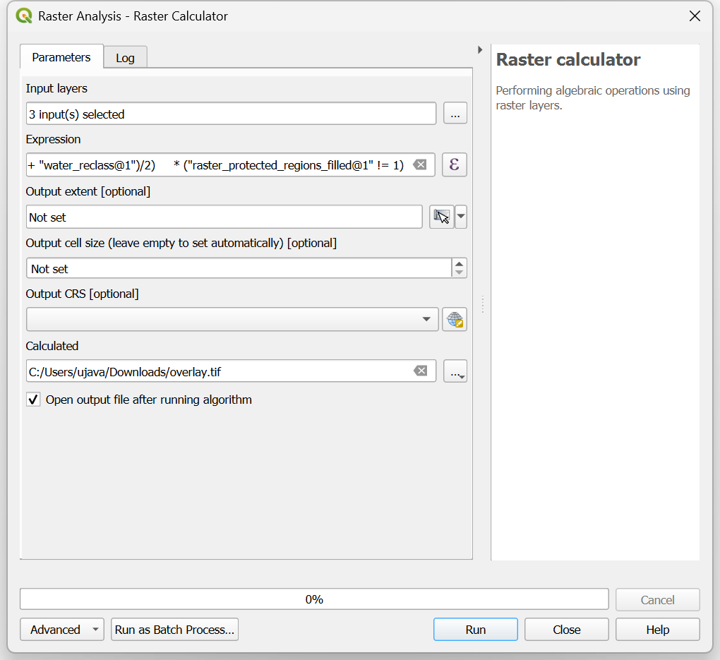

Opomba

In this example, we are giving equal weight to both road and water proximity. In real-life scenario, you may have multiple criteria with different importance. You can simulate that by multiplying the rasters with appropriate weights in the above expression. For example, if proximity to roads is twice as importance as proximity away from water, instead of (("roads_reclass@1" + "water_reclass@1")/2), you can use the expression ((2*"roads_reclass@1" + "water_reclass@1")/3).

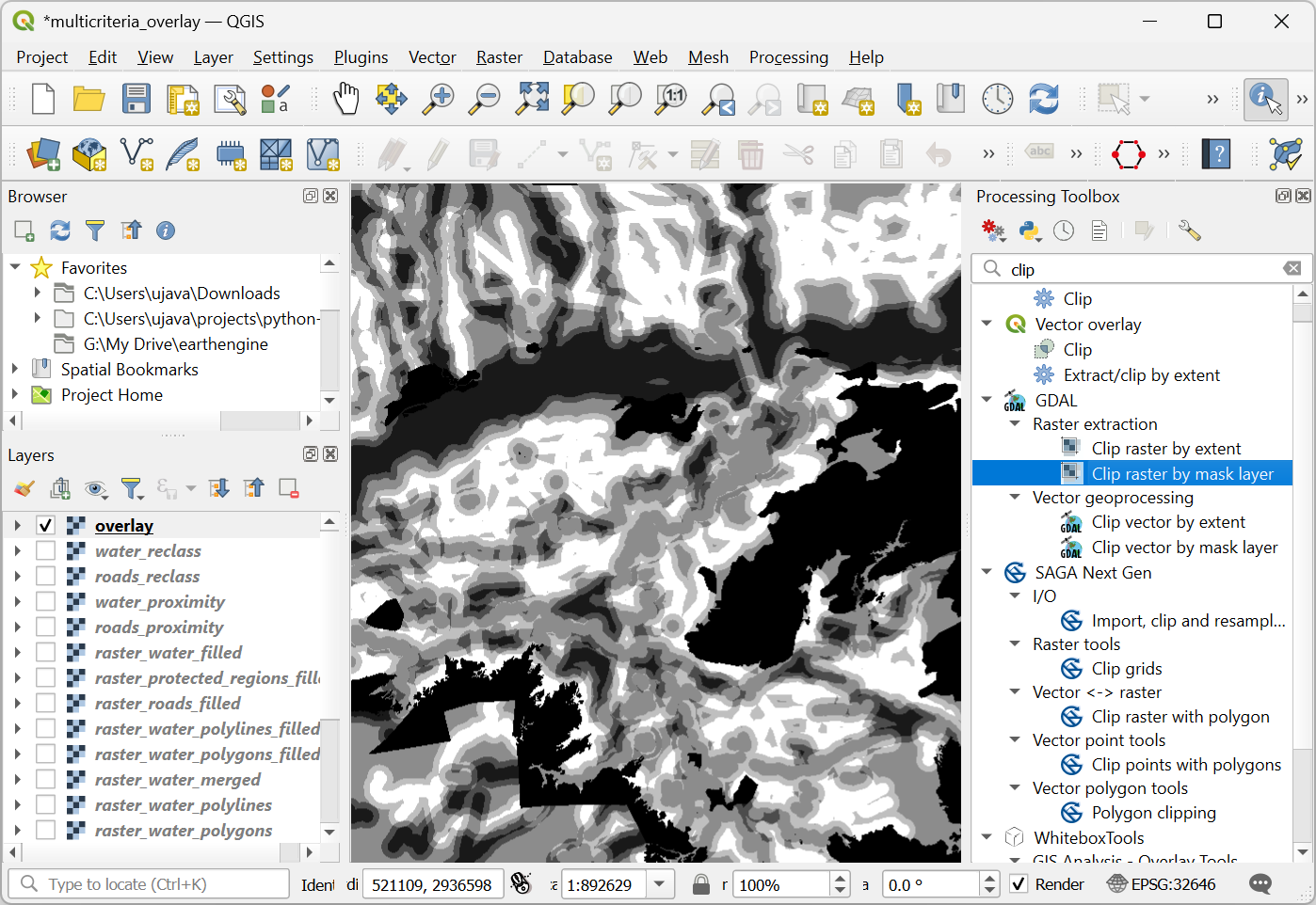
23. Once the processing finishes, the resulting raster overlay will be added to the Layers panel. The pixel values in this raster range from 0 to 100 - where 0 is the least suitable and 100 is the most suitable area for development. Let’s clip the results to the boundary layer. Open Raster extraction ‣ Clip raster by mask layer algorithm.

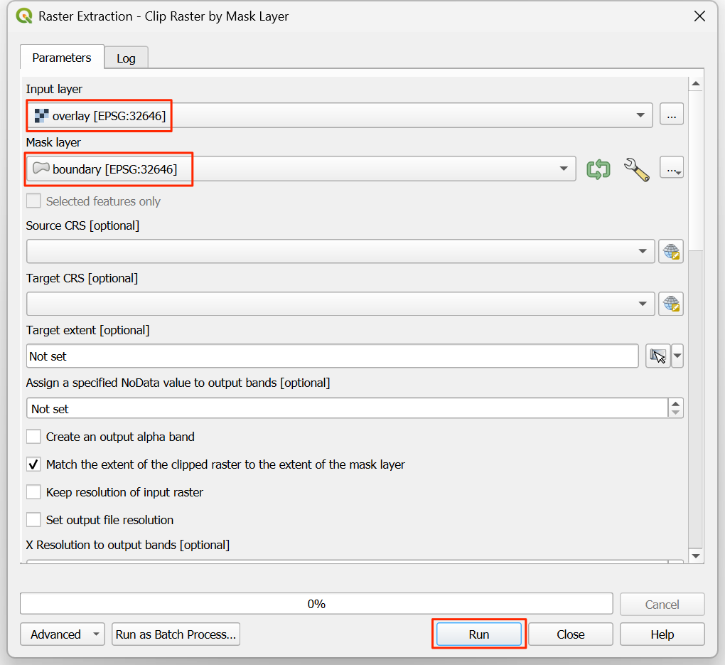
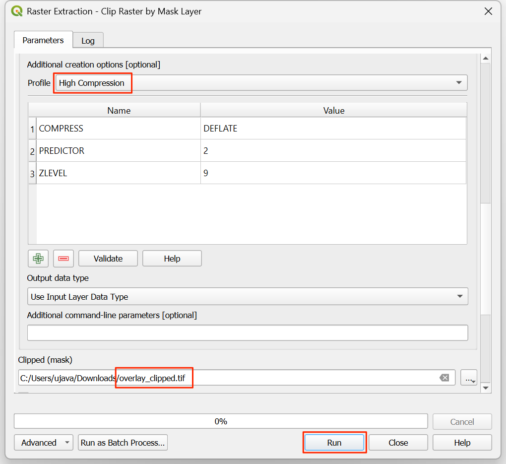
24. In the Raster Extraction - Clip Raster by Mask Layer dialog, select overlay as the Input layer and boundary as the Mask layer.

25. Scroll down to find the Advanced Parameters and select the profile High Compression to apply the compression. Save the Clipped (mask) layer as overlay_clipped.tif and click Run.

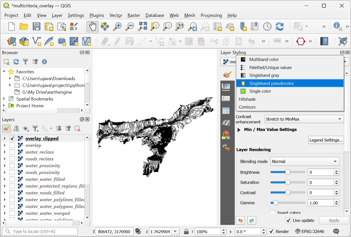
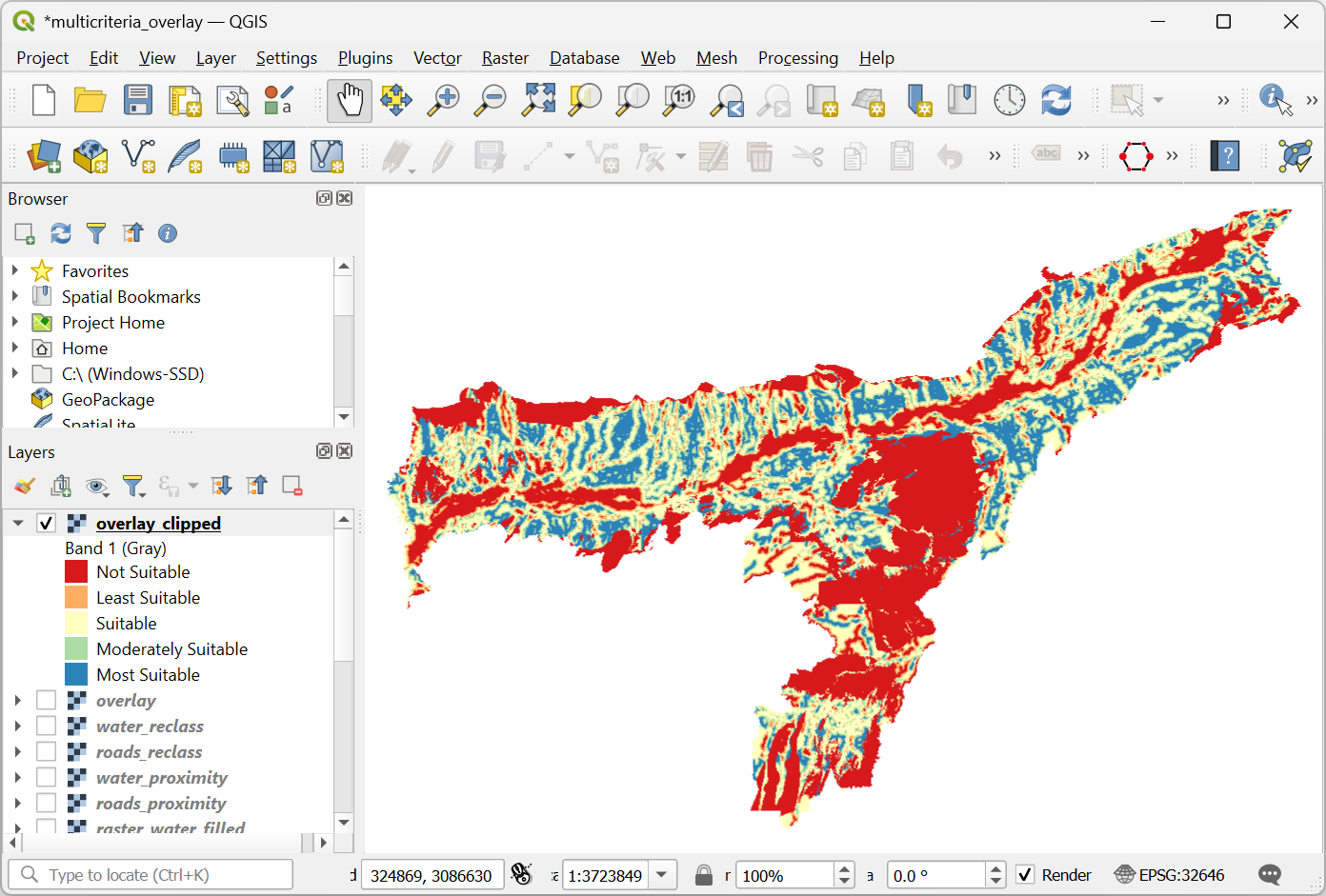
26. Once the processing finishes, the final output layer overlay_clipped will be added to the Layers panel. Click the Open the Layer Styling panel button in the Layers panel and select the Singleband pseudocolor renderer.

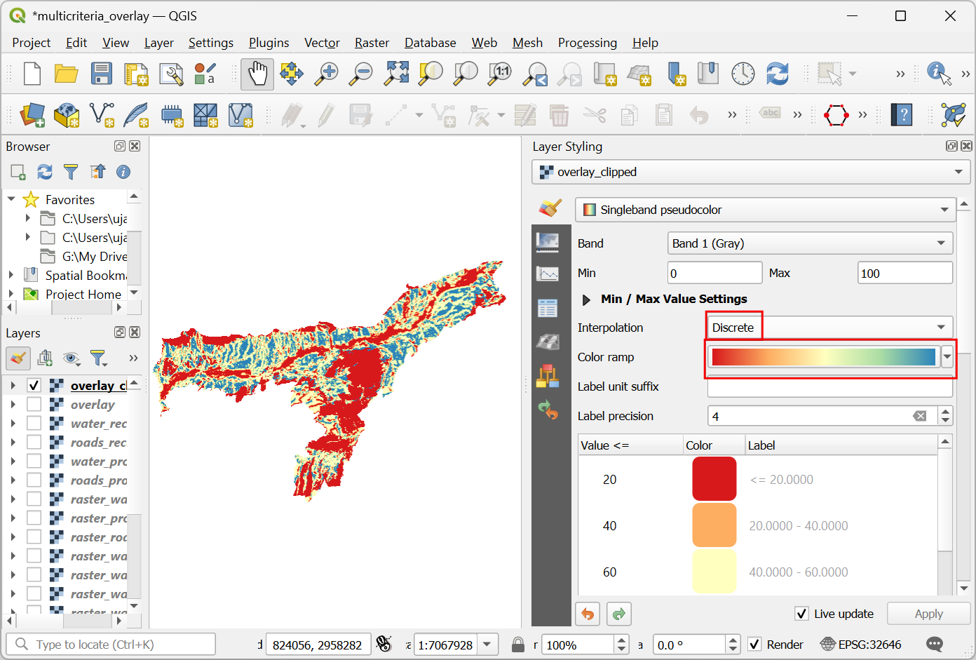
27. Set the Interpolation to Discrete and choose the Spectral color ramp.

28. Click on the default label values next to each color and enter appropriate labels.

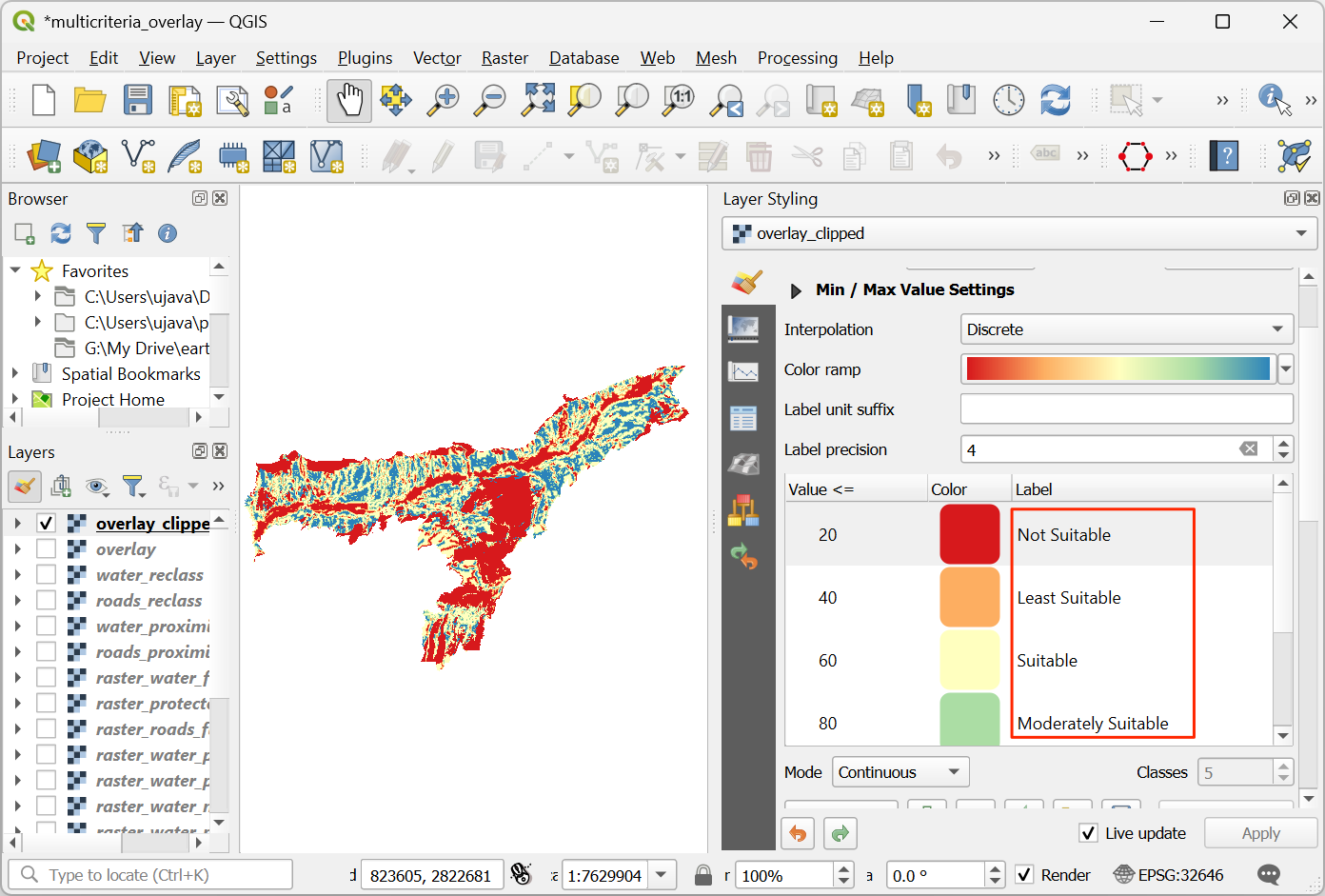
29. The labels will also appear as the legend under the overlay_clipped layer. This is our final map showing the site suitability according to the chosen criteria.

---

If you want to give feedback or share your experience with this tutorial, please comment below. (requires GitHub account)