Running Processing Algorithms via Python (QGIS3)

The Processing Toolbox in QGIS contain an ever-growing collection of geoprocessing tools. The toolbox provides an easy batch processing interface to run any algorithm on a large number of inputs. See 使用處理框架進行批次處理 (QGIS3). But there are cases where you need to incorporate a little bit of custom logic in your batch processing. As all the processing algorithms can be run programmatically via the Python API, you can run them via the Python Console. This tutorial shows how to run a processing algorithm via the Python Console to perform a custom geoprocessing task in just a few lines of code. Please review the Python 程式設計的初步上手 (QGIS3) tutorial to get familiar with the basics of the Python Scripting environment in QGIS.

Overview of the Task

We will use 12 gridded raster layers representing precipitation for each month of year and calculate average monthly rainfall for all zip codes in the Seattle area.

Other skills you will learn

• Access all layer(Raster and vector) from Python console and print their names.

• Merge diffrent layer into single layer using Python script.

Get the data

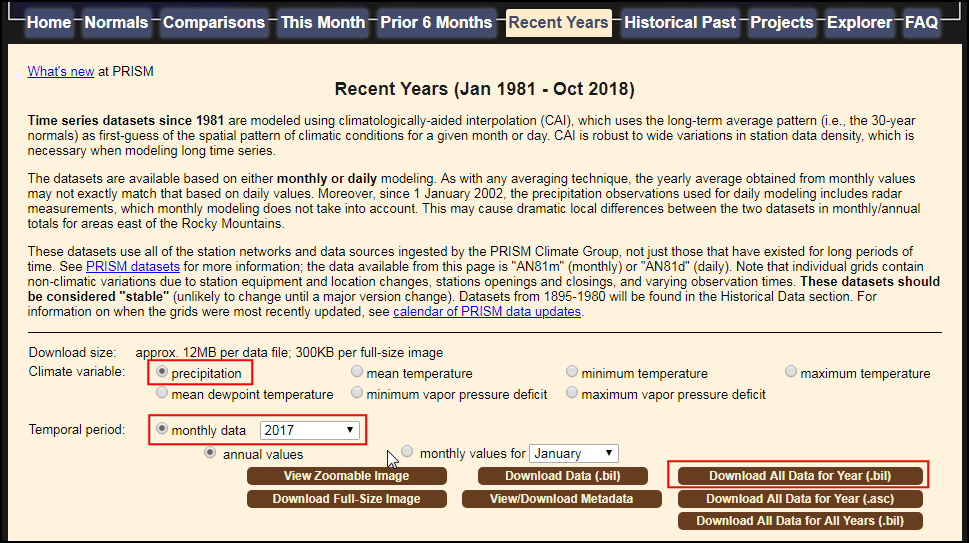
The PRISM Climate Group gathers climate observation and provides historic and current climate data for the conterminous US. Head over to the Recent Years data page and download the monthly precipitation data for the year 2017 in BIL format.

City of Seattle Open Data portal provides free and open data for the city. Search for and download the Zip Codes data in the shapefile format.

For convenience, you may directly download a copy of both the datasets from the links below:

PRISM_ppt_stable_4kmM3_2017_all_bil.zip

Zip_Codes.zip

Data Source [PRISM] [CITYOFSEATTLE]

Procedure

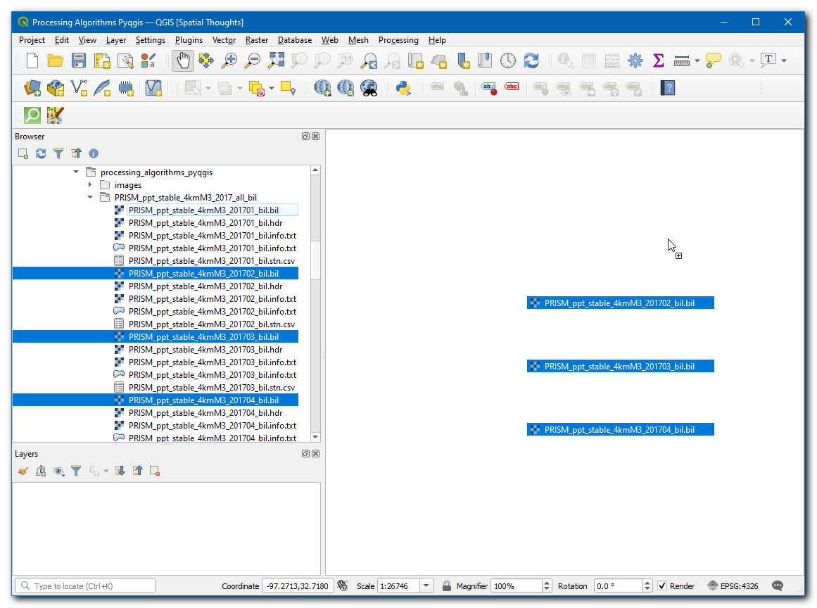
1. Locate the PRISM_ppt_stable_4kmM3_2017_all_bil.zip folder in the QGIS Browser and expand it. The folder contains 12 individual layers for each month. Hold the Ctrl key and select the .bil files for all 12 months. Once selected, drag them to the canvas.

備註

The data is provided in the BIL format. Each layer is presented with a set of files .bil file containing the actual data, a .hdr file describing the data structure and a .prj file containing the projection information. QGIS can load the .bil file and provided the other files exist in the same directory.

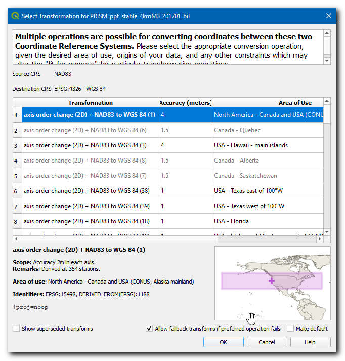
2. A Select Transformation of PRISM_ppt_stable_4kmM3_2017_all_bil dialog box will appear, leave the selection to default and click OK.

3. Next, locate the Zip_Codes.zip folder and expand it. Drag the Zip_Codes.shp file to the canvas.

4. Right-click the Zip_Codes layer and select Zoom to Layer. You will see the zip code polygons for the city of seattle and neighboring areas.

5. Go to Processing ‣ Toolbox.

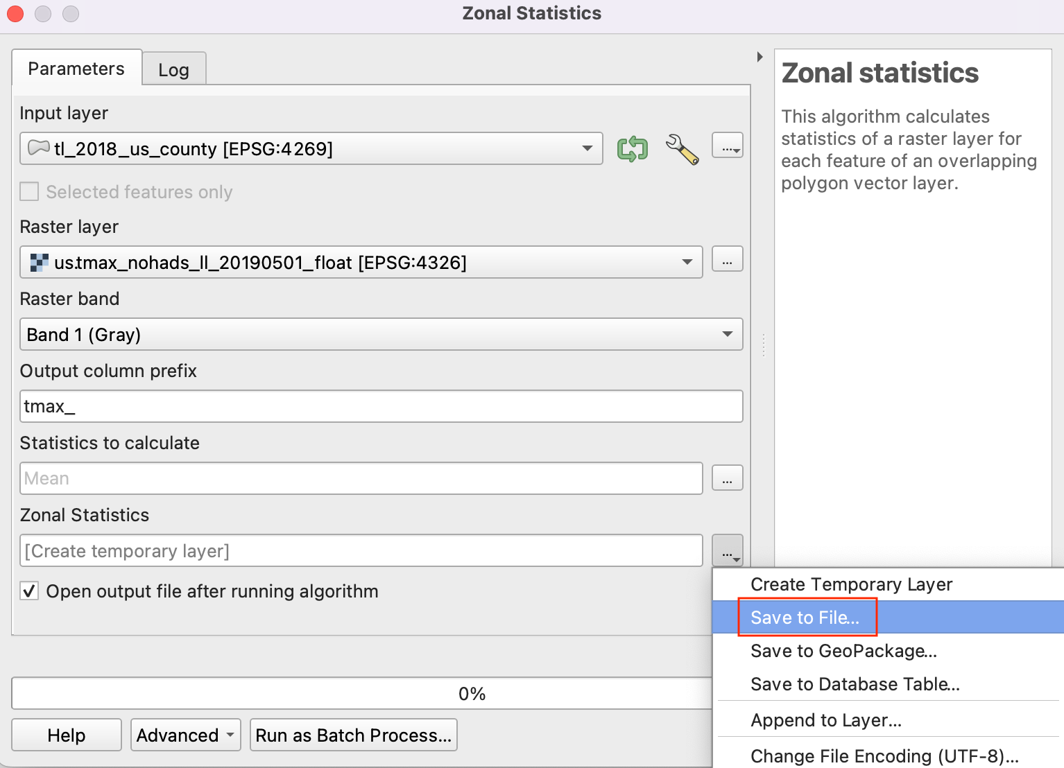
6. The algorithm to sample a raster layer using vector polygons is known as Zonal statistics. Search for the algorithm in the Processing Toolbox. Select the algorithm and hover your mouse over it. You will see a tooltip with the text Algorithm ID: 'native:zonalstatisticsfb'. Note this id which will be needed to call this algorithm via the Python API. Double-click the Zonal Statistics algorithm to launch it.

7. We will do a manual test run of the algorithm for a single layer. This is a useful way to check if the algorithm behaves as expected and also an easy way to find out how to pass on relevant parameters to the algorithm when using it via Python. In the Zonal Statistics dialog, select Zip_Codes as the Input layer PRISM_ppt_stable_4kmM3_201701_bil as the Raster Layer and, leave other parameters to default. Click the ... button next to Statistics to calculate and select only Mean, next click the ... button next to Zonal Statistics and save the layer as january_mean.gpkg Click Run .

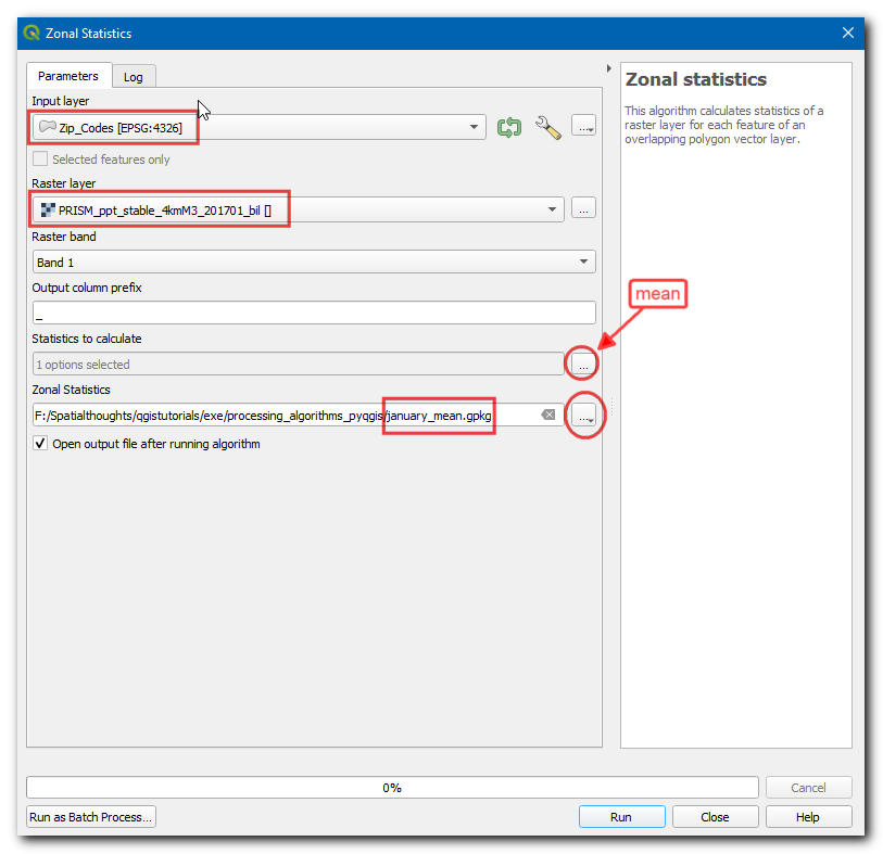
8. Once the algorithm finishes, switch to the Log tab. Make a note of the Input Parameters that were passed to the algorithm. Click Close.

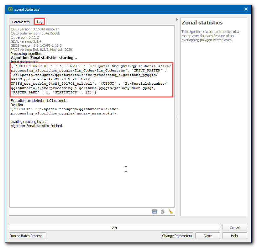
9. Now a new layer january_mean will be added to the canvas. Let's check the results, right-click on the layer and select Open Attribute Table. This particular algorithm modifies the input zone layer in-place and adds a new column for every statistic that was selected. As we had selected only Mean value, a new column named _mean is added to the table. The _ was the default prefix. When we run the algorithm for layers of each month, it will be useful to specify a custom prefix with the month number so we can easily identify the mean values for each month (i.e. 01_mean, 02_mean etc.). Specifying this custom prefix is not possible in the Batch Processing interface of QGIS and if we ran this command using that interface, we would have to manually enter the custom prefix for each layer. If you are working with a large number of layers, this can be very cumbersome. Hence, we can add this custom logic using the Python API and run the algorithm in a for-loop for each layer.

10. Back in the main QGIS window, go to Plugins ‣ Python Console.

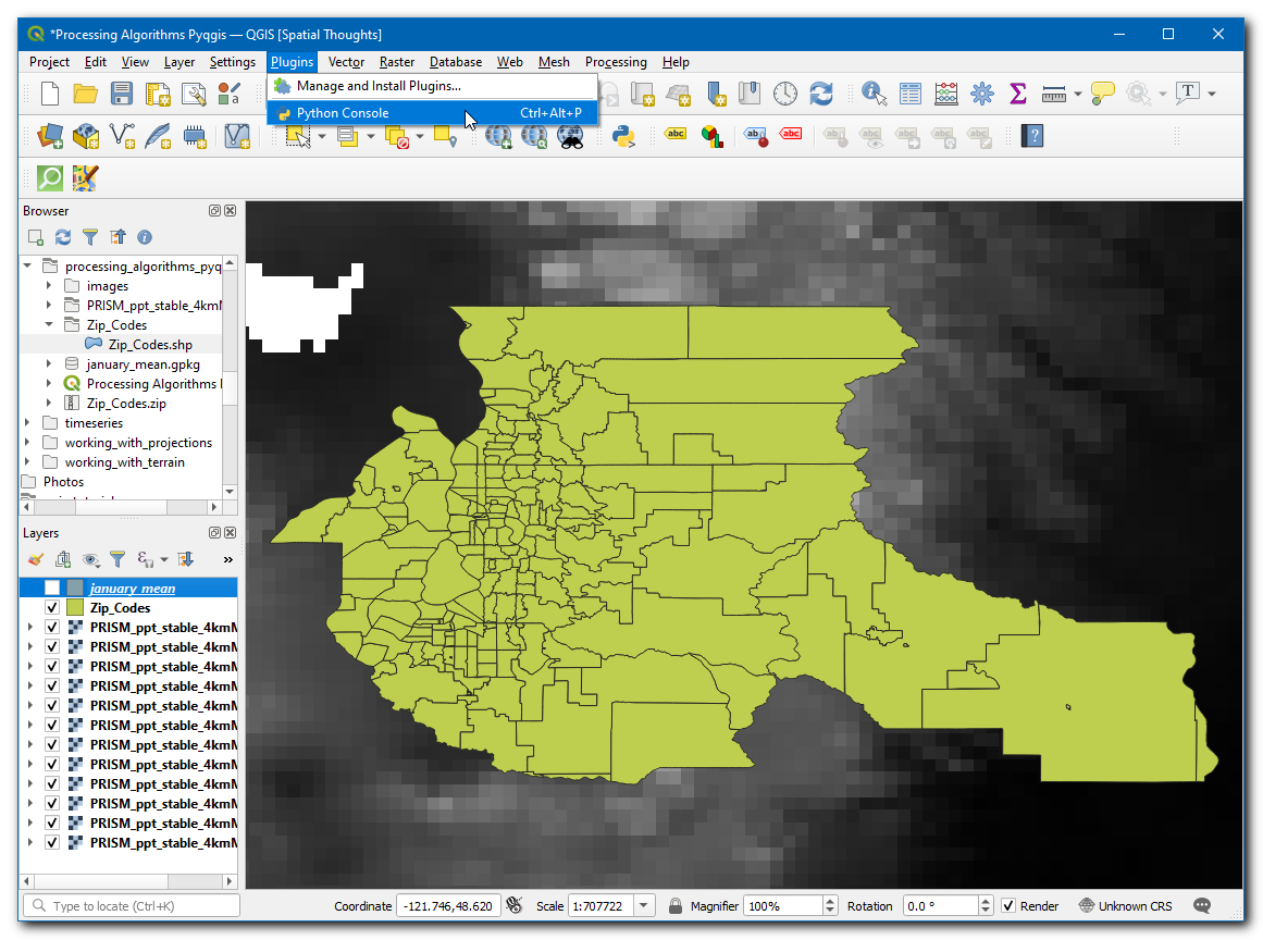
11. Click on the show editor button. This will open the python editor where a bunch of python code can be written and executed with a single click of a button.

12. To run the processing algorithm via Python, we need to access names of all the layers. Enter the following code in the editor and click on the Play button. You will see the names of all layers printed in the console.

root = QgsProject.instance().layerTreeRoot()
for layer in root.children():
  print(layer.name())

13. Now, let's calculate the Mean for one month and create an output layer. In the below code break is used to exit the loop after the first execution, by this we can calculate the mean for January month.

import re

root = QgsProject.instance().layerTreeRoot()

input_layer = 'Zip_Codes'
unique_field = 'OBJECTID'

# Iterate through all raster layers
for layer in root.children():
  if layer.name().startswith('PRISM'):
    # Run Zonal Stats algorithm
    # Extract the YYYYMM part of the layer name
    pattern = r'_(\d+)_'
    matches = re.findall(pattern, layer.name())
    # Use the month as the prefix
    prefix = matches[0][-2:]
    params = {'INPUT_RASTER': layer.name(),
        'RASTER_BAND': 1, 'INPUT': input_layer,
        'COLUMN_PREFIX': prefix+'_', 'STATISTICS': [2],
        'OUTPUT': 'memory:'
        }
    result = processing.run("native:zonalstatisticsfb", params)

    result_layer = result['OUTPUT']
    QgsProject.instance().addMapLayer(result_layer)
    # Breaking out of loop to demonstrate the
    # zonalstatistics algorithm.
    break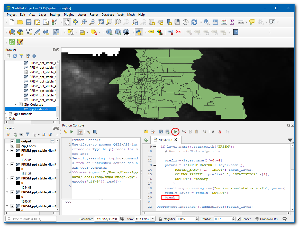

備註

You can also run a QGIS Processing algorithm via Python using the processing.runAndLoadResults() function instead of processing.run() as shown above - which will load the result to QGIS canvas directly.

14. A new layer output will be added to the canvas, right-click on the layer and select Open Attribute Table. 01_mean represents one month mean, likewise the above algorithm will produce 12 new layers if executed without the break.

15. Now lets add code to merge all the months mean, and create an single output layer from it. We update the previous code, to iteratively run the Zonal Statistics algorithm. We define a new variable result_layer which is set to Zip_Codes in the beginning but gets updated with the output layer from each iteration. This will allow us to use the result of each iteration and add new columns to it. Enter the following code to iterate over all raster layers and create an single layer containing all months mean.

import re

root = QgsProject.instance().layerTreeRoot()

input_layer = 'Zip_Codes'
result_layer = input_layer
unique_field = 'OBJECTID'

# Iterate through all raster layers
for layer in root.children():
  if layer.name().startswith('PRISM'):
    # Run Zonal Stats algorithm
    # Extract the YYYYMM part of the layer name
    pattern = r'_(\d+)_'
    matches = re.findall(pattern, layer.name())
    # Use the month as the prefix
    prefix = matches[0][-2:]
    params = {'INPUT_RASTER': layer.name(),
        'RASTER_BAND': 1, 'INPUT': result_layer,
        'COLUMN_PREFIX': prefix+'_', 'STATISTICS': [2],
        'OUTPUT': 'memory:'
        }
    result = processing.run("native:zonalstatisticsfb", params)

    # Update the result_layer variable
    # The result will be used as input for the next iteration
    result_layer = result['OUTPUT']

QgsProject.instance().addMapLayer(result_layer)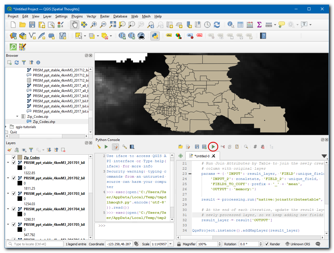

16. Once the processing finishes, a new layer output will be added to canvas, right-click on the layer and select Open Attribute Table.

17. You will see 12 new columns added to the table with custom prefixes and mean precipitation values extracted from the raster layers.

---

If you want to give feedback or share your experience with this tutorial, please comment below. (requires GitHub account)