為紙本地圖進行空間對位 (QGIS3)

大部分的 GIS 專案都會需要對某些影像進行「 空間對位 （Georeferencing） 」，也就是說要為影像的每個像素指定它在世界上的地理空間座標。在許多的情況下，這些座標是透過野外調查收集而來，例如說用 GPS 裝置定位那些易於辨識的地標。但有的時候，例如說如果你要使用的是某地圖的數位化掃描檔，你也可以藉由地圖上的一些標記來蒐集空間座標。一旦我們有了這些採樣的座標點或地面控制點 (Ground Control Points)，這些影像就可以用給定的座標系統來投影繪製。在本章節中，我們會討論相關的概念、作法與 QGIS 提供的工具，以達成高準確度空間對位的目標。

本教學的目標是為一張具有座標資訊 (例如有座標標切的經緯度網格) 的地圖影像進行空間對位。如果你的來源影像沒有這類資訊，請參考在 為空照圖進行空間對位 (QGIS3) 中的說明。

內容說明

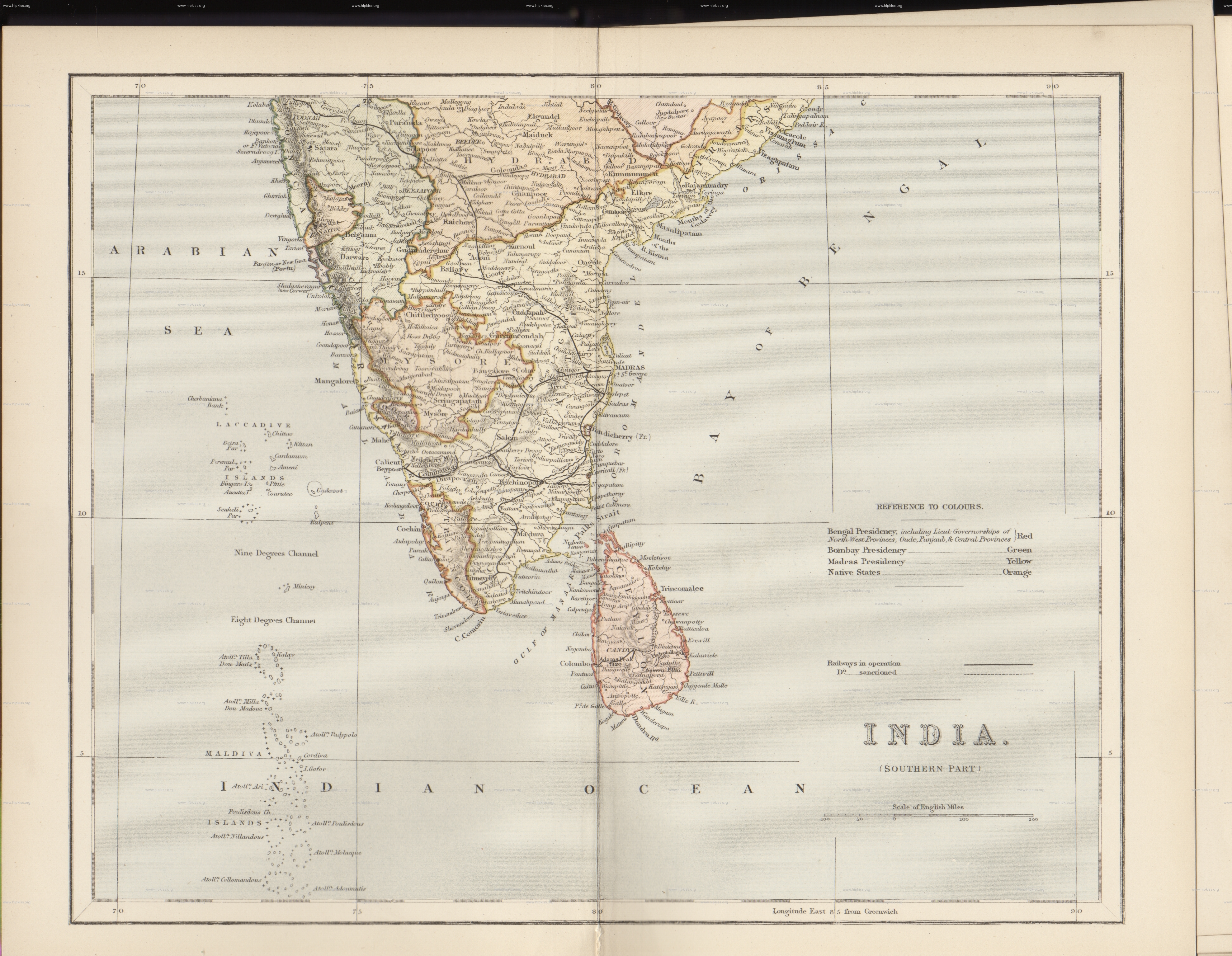
我們要為一份 1870 年的南印地圖掃描檔，以 QGIS 進行空間對位。

你還會學到這些

• 如何判斷老地圖的大地座標（Datum）與座標系統（Coordinate System）。

• Save the GCP created.

• Edit the created GCP for fine tuning.

取得資料

Hipkiss’s Scanned Old Maps 網站蒐集了不少版權過期的老地圖掃描檔，非常適合用在研究上。

這邊可以下載儲存 1870 年的南印度地圖 的 JPG 檔。

為了方便起見，你也可以直接用下面的連結下載：

1870_southern_india.jpg

操作流程

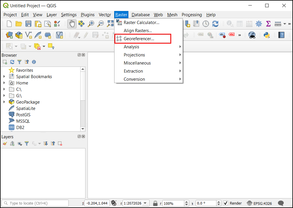
1. Open QGIS and click on Raster ‣ Georeferencer to open the tool.

備註

From QGIS versions 3.26 onwards, the Georeferencer can be launched from Layer ‣ Georeferencer.

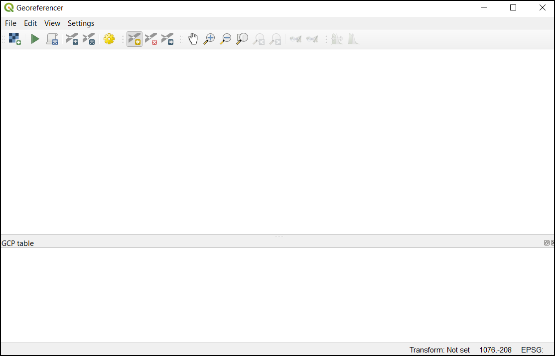
2. The Georeferencer is divided into 2 sections. The top section where the image will be displayed and the bottom section where a table showing your GCPs will appear.

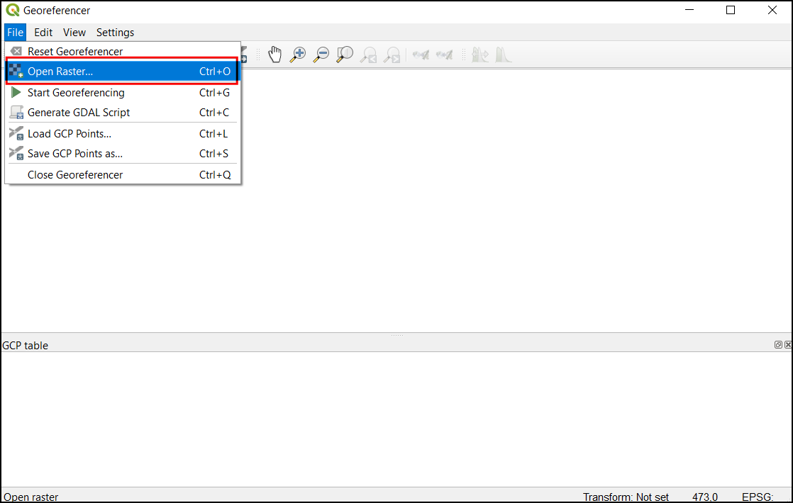
3. 現在就來開啟我們的 JPG 影像。選擇 檔案 ‣ Open Raster，然後找到剛才下載的地圖掃描檔，按下 開啟舊檔。

4. 現在影像已經被載到螢幕上半部了。可以使用工具列的放大/平移功能觀察一下地圖的細節。

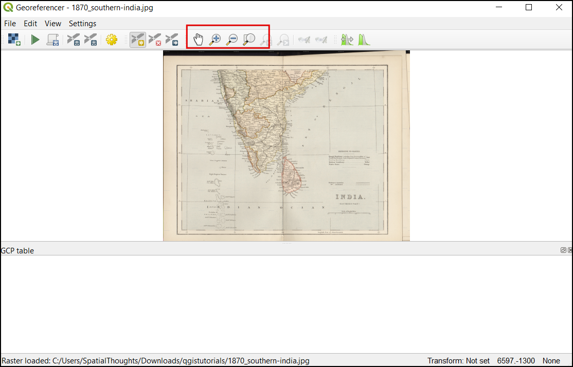
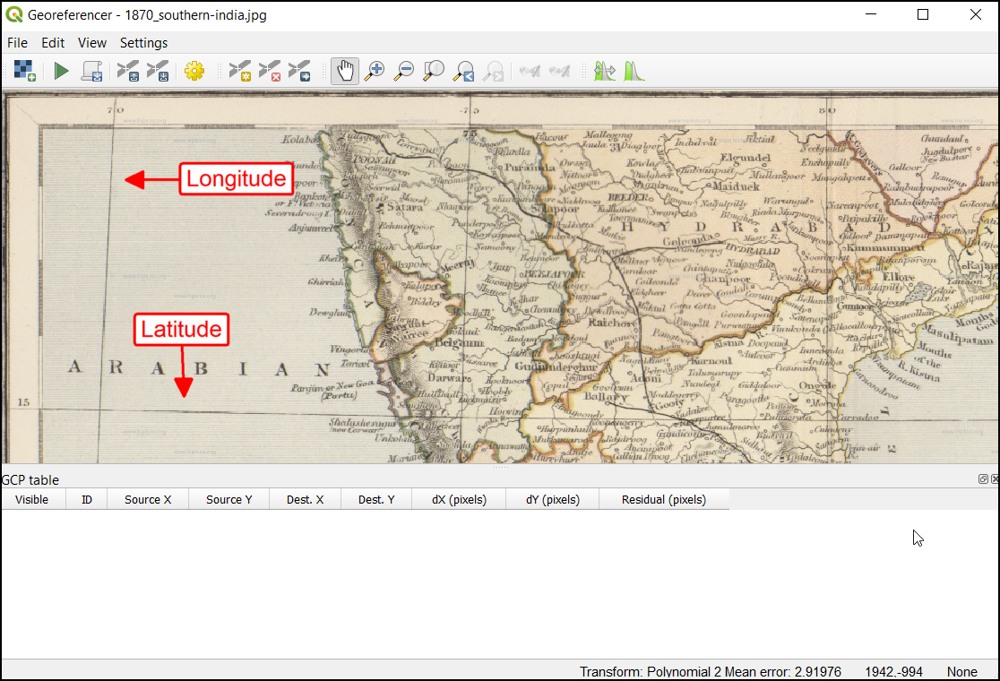
5. 現在我們要為圖上的某些點指定座標了。仔細觀察後，可以發現本地圖具有標示經緯度的格線。

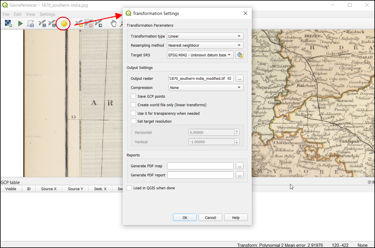
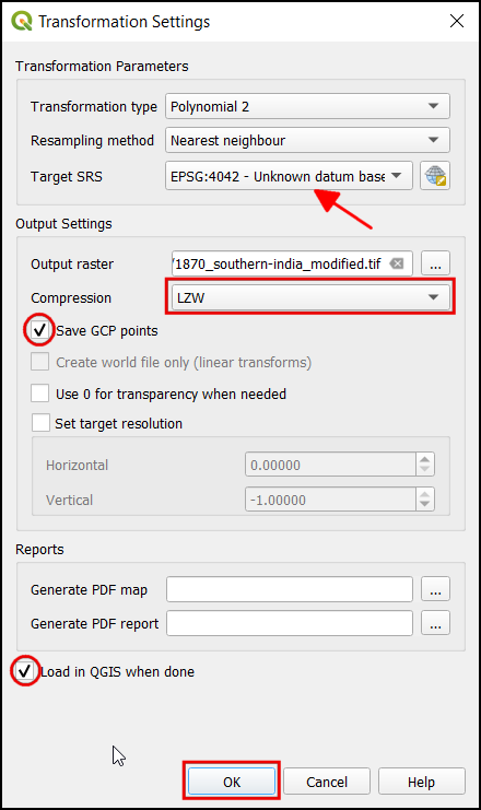
6. Before adding Ground Control Points (GCP), we need to define the Transformation Settings. Click on the gear icon in georeferencing window to open the Transformation settings dialog.

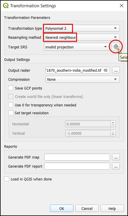
7. In the Transformation settings dialog, choose the Transformation type as Polynomial 2. See QGIS Documentation to learn about different transformation types and their uses. Then select the Resampling method as the Nearest neighbor. Click the Select CRS button next to Target SRS.

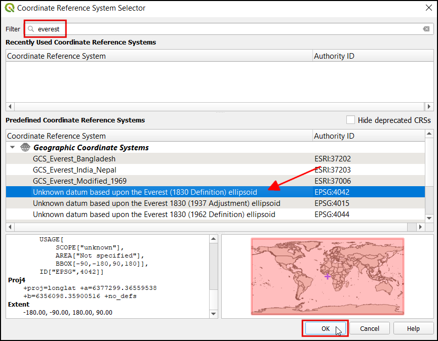
8. 在本例的情況下，CRS 資訊可以直接在地圖影像掃描檔上取得。我們先端詳一下地圖，可發現本地圖的座標是經緯度，不過並沒有標示任何的大地座標系統資訊，所以我們得自己假設一個才行。因為此地圖是年代久遠的印度地圖，我們可以猜測它是使用 Everest 1830 大地座標系統，這應該會有不錯的結果。搜尋 everest 然後選擇最老的 Everest 大地基準的 CRS (EPSG:4042)，然後按下 OK。

備註

Survey of India Topo Sheets created between the year 1960 and 2000 use the Everest 1956 spheroid and India_nepal datum. If you are georeferencing SOI Topo Sheets, , you can define a Custom CRS in QGIS with the following paramters and use it in this step. This definition includes a delta_x, delta_y and delta_z parameters for transforming this datum to WGS84. See this page for more information on the Indian Grid System.

+proj=longlat +a=6377301.243 +b=6356100.2284 +towgs84=295,736,257,0,0,0,0 +no_defs

備註

Most maps are created using a Projected CRS. If the map you are trying to georeference uses a projected CRS that you know of, but the graticules labels are in a Geographic CRS (latitude/longitude), you may use an alternate workflow to minimize distortion. Instead of using a Geographic CRS like we are using here, you can create a vector grid in QGIS and transform it to the projected CRS to be used as a reference for accurate coordinate capture. See this page for more details.

9. Name your output raster as 1870_southern_india_modified.tif. Choose LZW as the Compression. Check the Save GCP points to store the points as seperate file for future purpose. Make sure the Load in QGIS when done option is checked. Click OK.

備註

Uncompressed GeoTIFF files can be very large in size. So compressing them is always a good idea. You can learn more about different TIFF compression options (LZW, PACKBITS or DEFLATE) in this article.

10. Now we can start adding the Ground Control Points (GCP). Click on the Add Point button.

11. Now place the cross-hair at the intersections of the grid lines and left-click, this will serve as the ground-truth in our case. As the grid lines are labeled, we can determine the X and Y coordinates of the points using them. In the pop-up window, enter the coordinates. Remember that X=longitude and Y=latitude. Click OK.

12. 這下子，下半部的地面控制點表格會新增一欄你剛剛選的地面控制點。

13. Similarly, add more GCPs covering the entire image. The more points you have, the more accurate your image is registered to the target coordinates. The Polynomial 2 transform requires at least 6 GCPs. Once you have added the minimum number of points required for the transform, you will notice that the GCPs now have a non-zero dX, dY and Residual error values. If a particular GCP has unusually high error values, that usually means a human-error in entering the coordinate values. So you can delete that GCP and capture it again. You can also edit the coordinate values in the GCP Table by clicking the cell in either Dest. X or Dest. Y columns.

14. Once you are satisfied with the GCPs, click the Start Georeferencing button. This will start the process of warping the image using the GCPs and creating the target raster.

15. Once the process finishes, you will see the georeferenced layer loaded in QGIS. The georeferencing is now complete. Also, you will notice the Project CRS in the bottom right is set to EPSG:4042 as described in Transformation Settings.

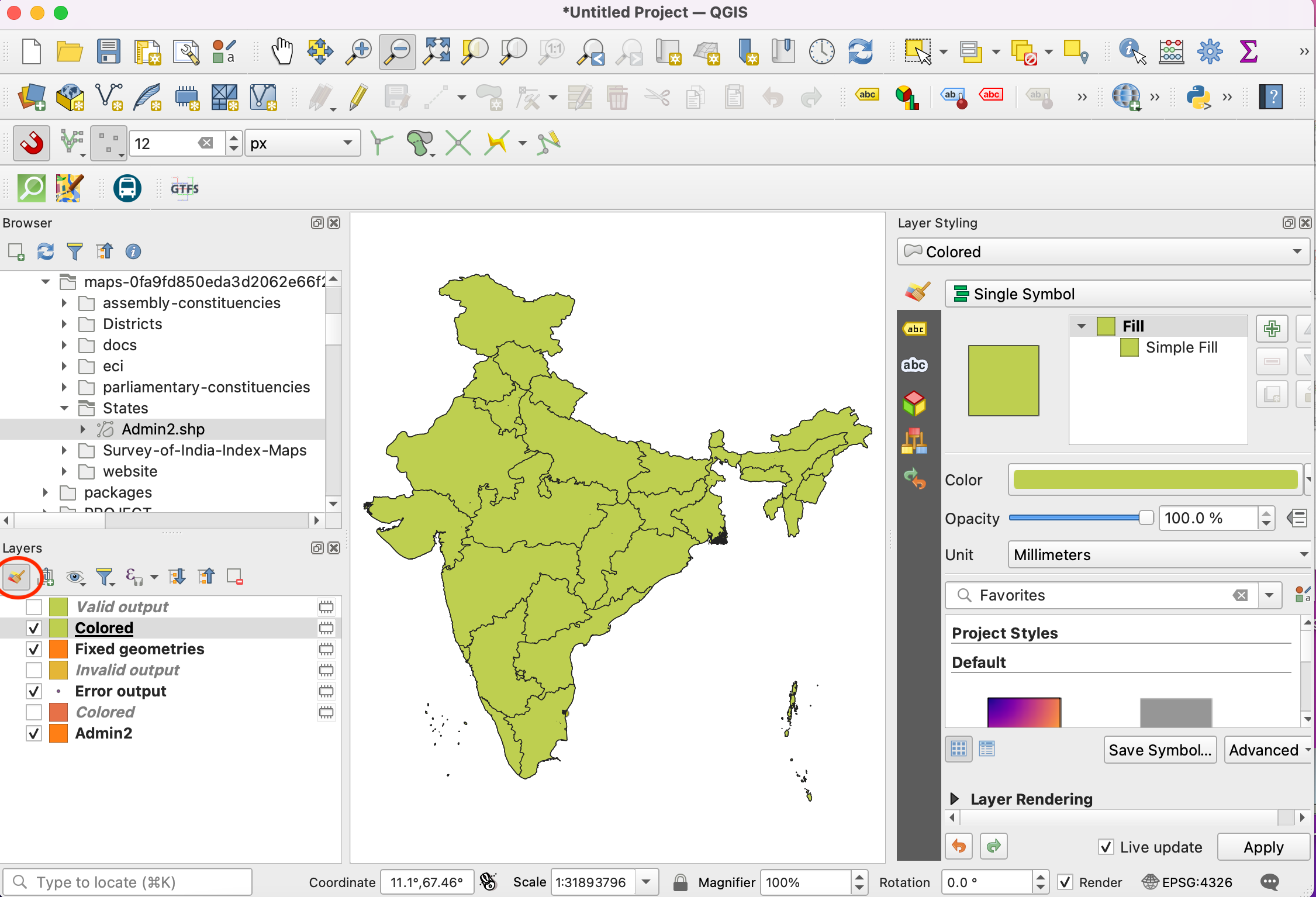
16. Drag and drop the OpenStreetMap as Base Map from the XYZ Tiles dropdown at the bottom of the Browser panel to verify the georeferenced layer. To set the transparency, click on the Open layer styling panel icon and select Transparency tab. Set the transparency to 40 %. Now the georeferenced image must overlay with the basemap outline.

17. If the georeference needs more fine-tuning, we can start from the collected GCP points. Browse the 1870_southern_india_modified.tif file location. You can find an additional file, 1870_southern_india_modified.tif.points. This file will contain the GCP points information.

18. Open the georeferencing tool in QGIS, click File ‣ Load GCP Points, and select the 1870_southern_india_modified.tif.points. This will load the GCP created previously. Then load the 1870_southern_india_modified.tif to fine-tune your work.

---

If you want to give feedback or share your experience with this tutorial, please comment below. (requires GitHub account)