 Ujaval Gandhi
Avtomatizacija ustvarjanja zemljevidov s programom Print Layout Atlas (QGIS3)
Če vaša organizacija objavlja tiskane ali spletne zemljevide, boste pogosto morali ustvariti več zemljevidov z isto predlogo - običajno po enega za vsako upravno enoto ali interesno območje. Ročno ustvarjanje teh zemljevidov lahko traja dolgo in če jih želite redno posodabljati, je to lahko zelo naporno. QGIS ima orodje, imenovano Atlas, ki vam lahko pomaga ustvariti predlogo zemljevida in enostavno objavo velikega število zemljevidov za različne geografske regije. Če niste seznanjeni z osnovami postavitve tiskanja, si preberite Ustvarjanje karte tutorial.
Pregled naloge
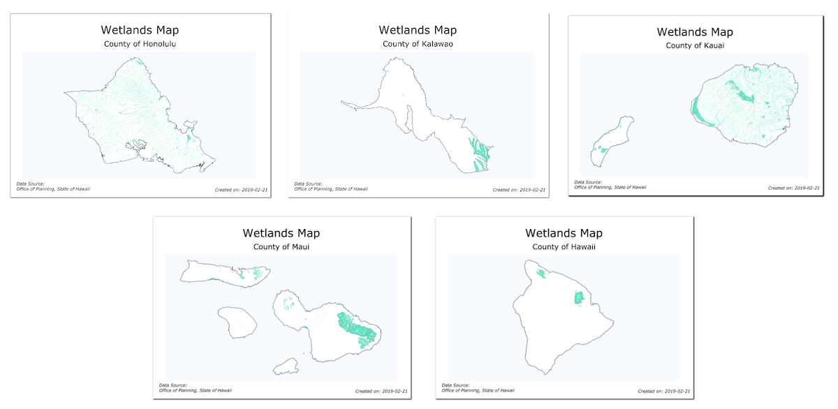
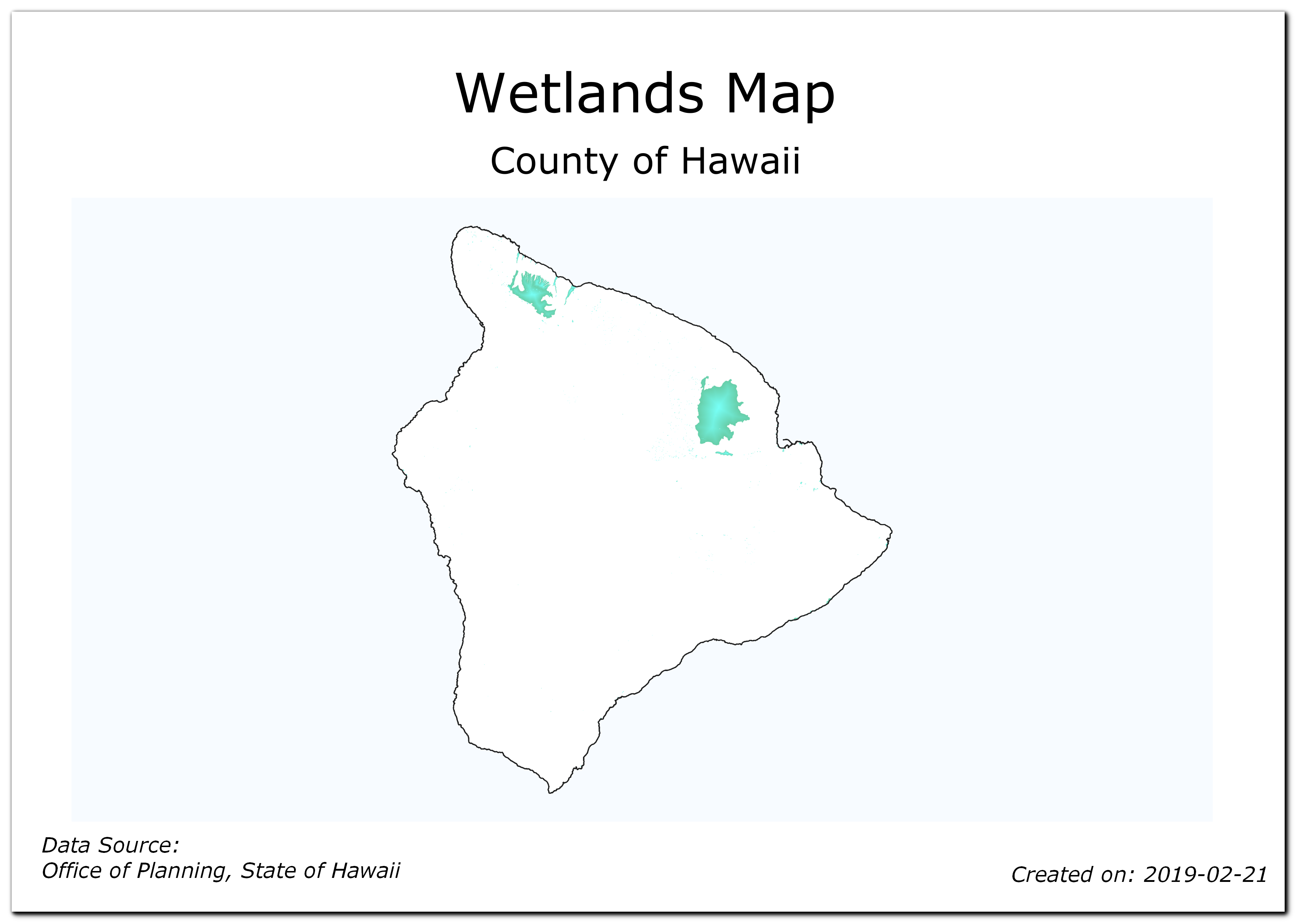
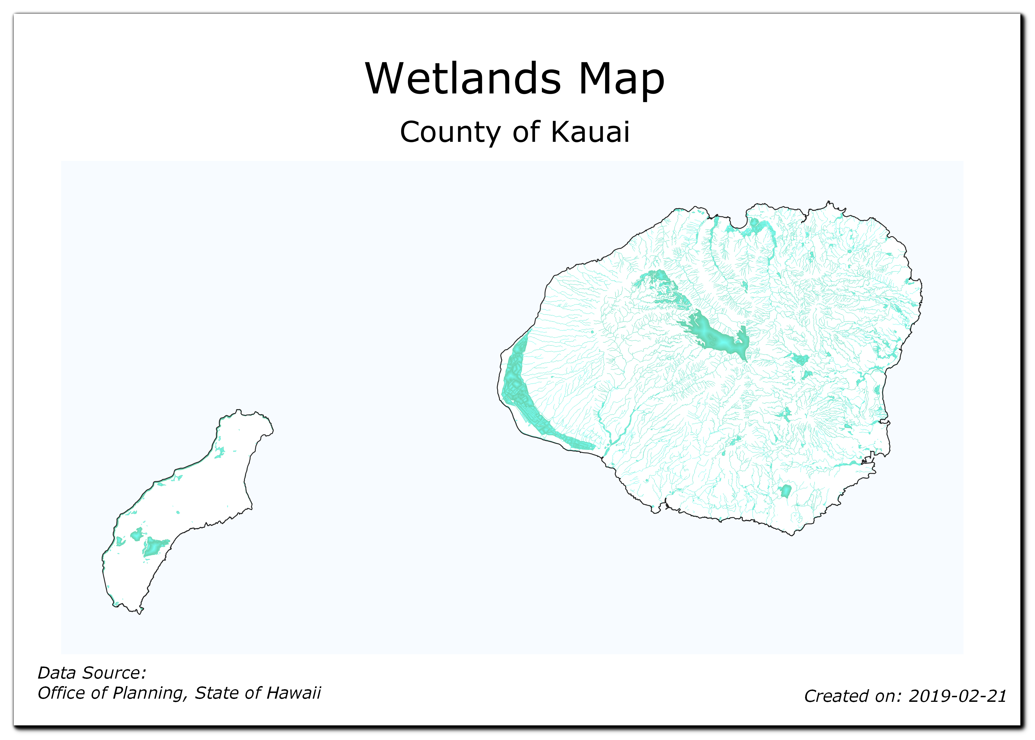
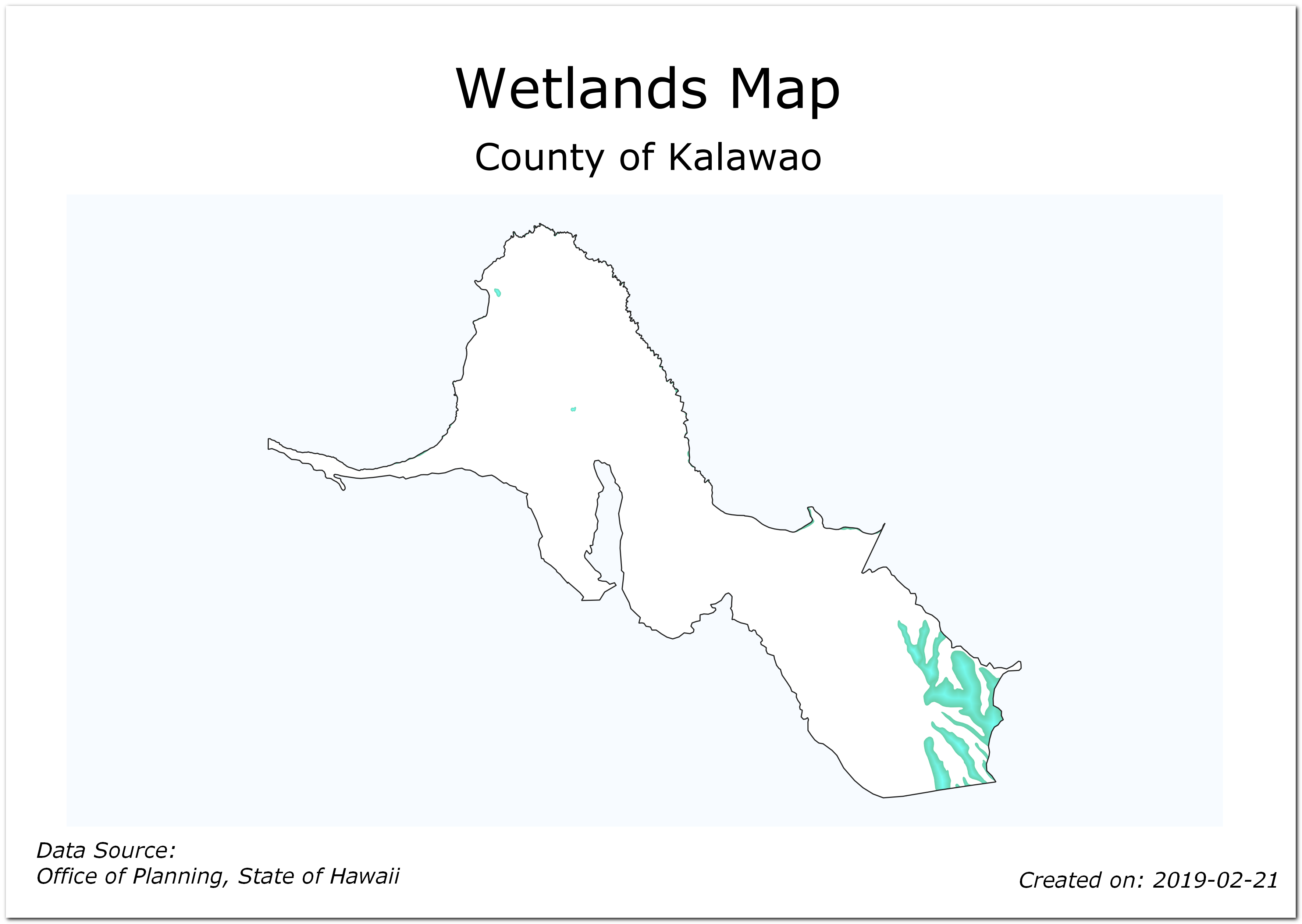
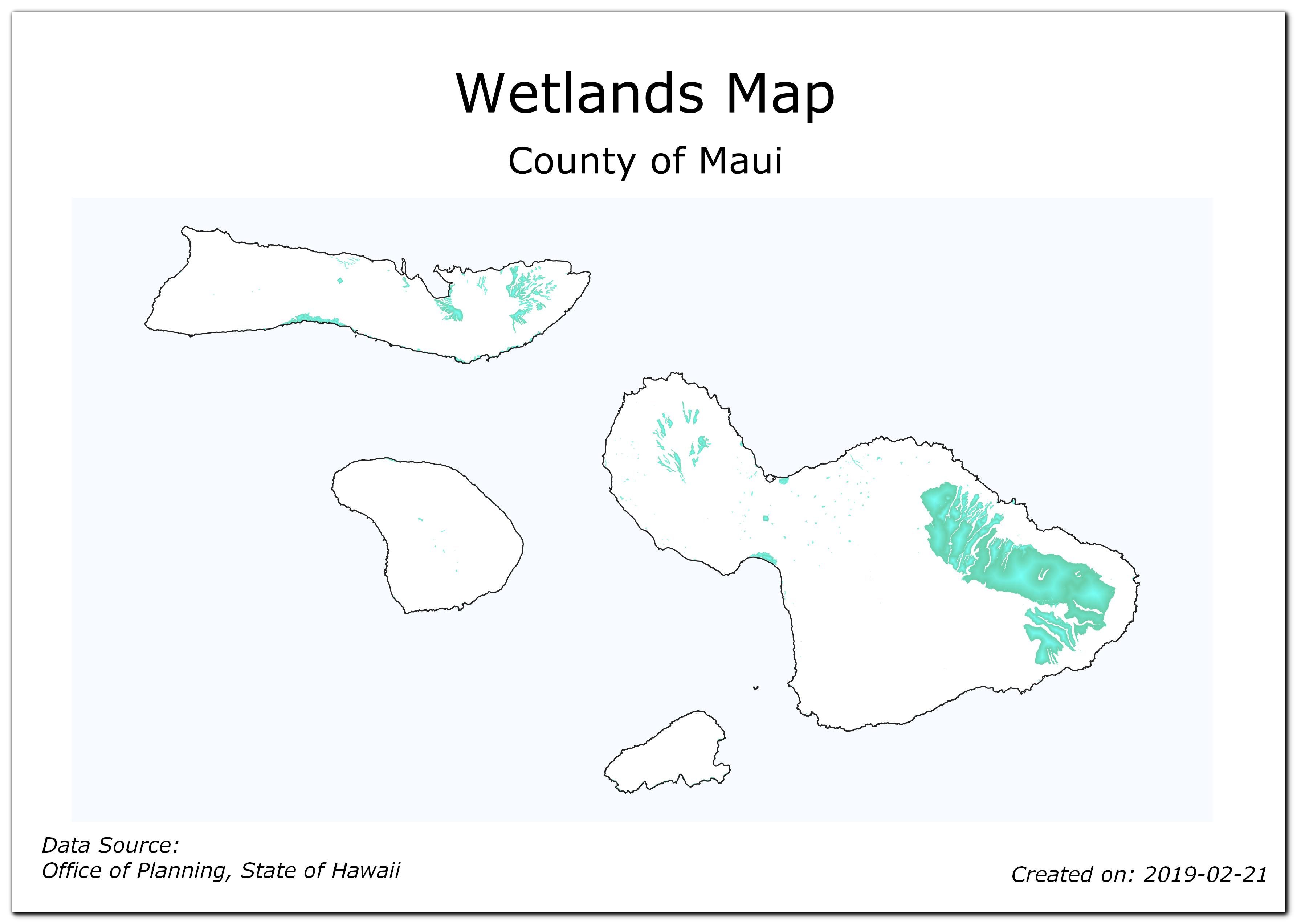
Ta vadnica prikazuje, kako ustvariti zemljevid mokrišč za vsako okrožje v zvezni državi Havaji.
Druga znanja, ki jih boste pridobili
Uporaba prikazovalnika v slogu
Invertirani poligoniza zapolnitev območij zunaj poligonov.Napišite izraz v prikazovalniku sloga
Rule Basedza prikaz samo trenutne funkcije v Atlasu.Napišite izraz za ustvarjanje dinamičnih oznak v postavitvi za tiskanje.
Uporaba upodobitvenega sloga
Shapeburst fillza ustvarjanje dvobarvnega poligonskega polnila.
Pridobivanje podatkov
Uporabili bomo podatkovne sloje GIS iz State of Hawaii - Office of Planning
Prenesite sloj Močvirja iz kategorije Biologic and Ecologic.
Prenesite sloj Census County Boundaries 2010 iz kategorije Kulturni in demografski podatki.
Zaradi priročnosti lahko kopijo obeh zbirk podatkov neposredno prenesete s spodnjih povezav:
Vir podatkov [HAWAII]
Postopek
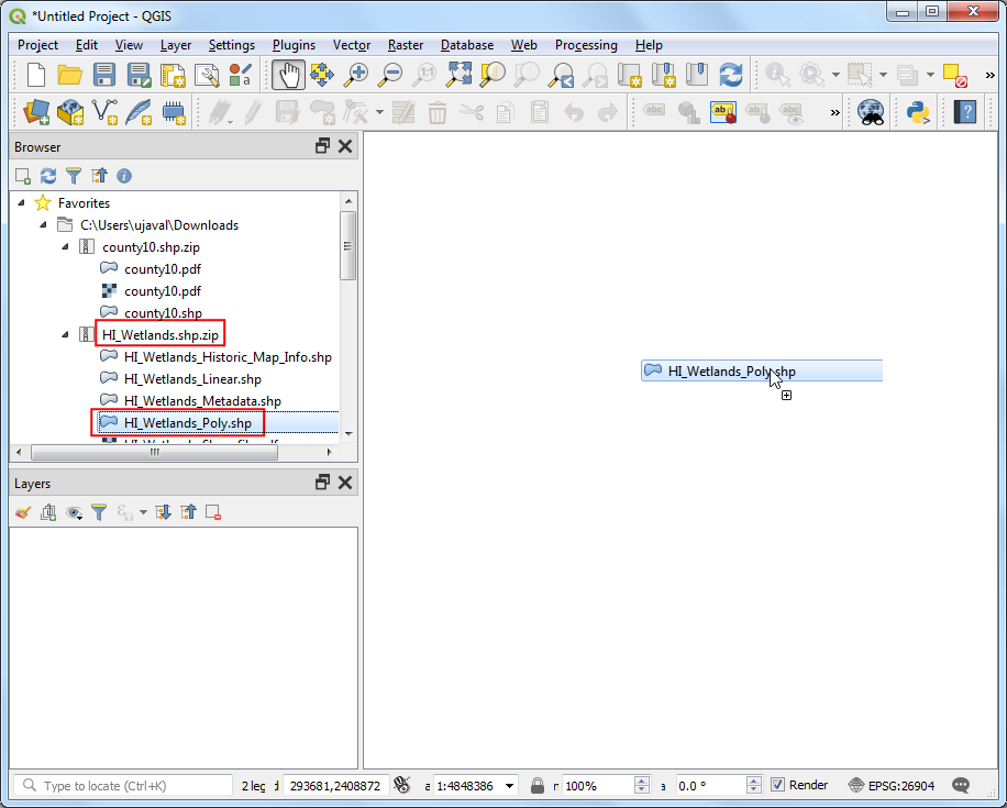
V brskalniku QGIS poiščite datoteko
HI_Wetlands.shp.zipin jo razširite. Izberite datotekoHI_Wetlands_Poly.shpin jo povlecite na deovno površino. Ta sloj vsebuje poligone, ki predstavljajo mokrišča v celotni državi Havaji.
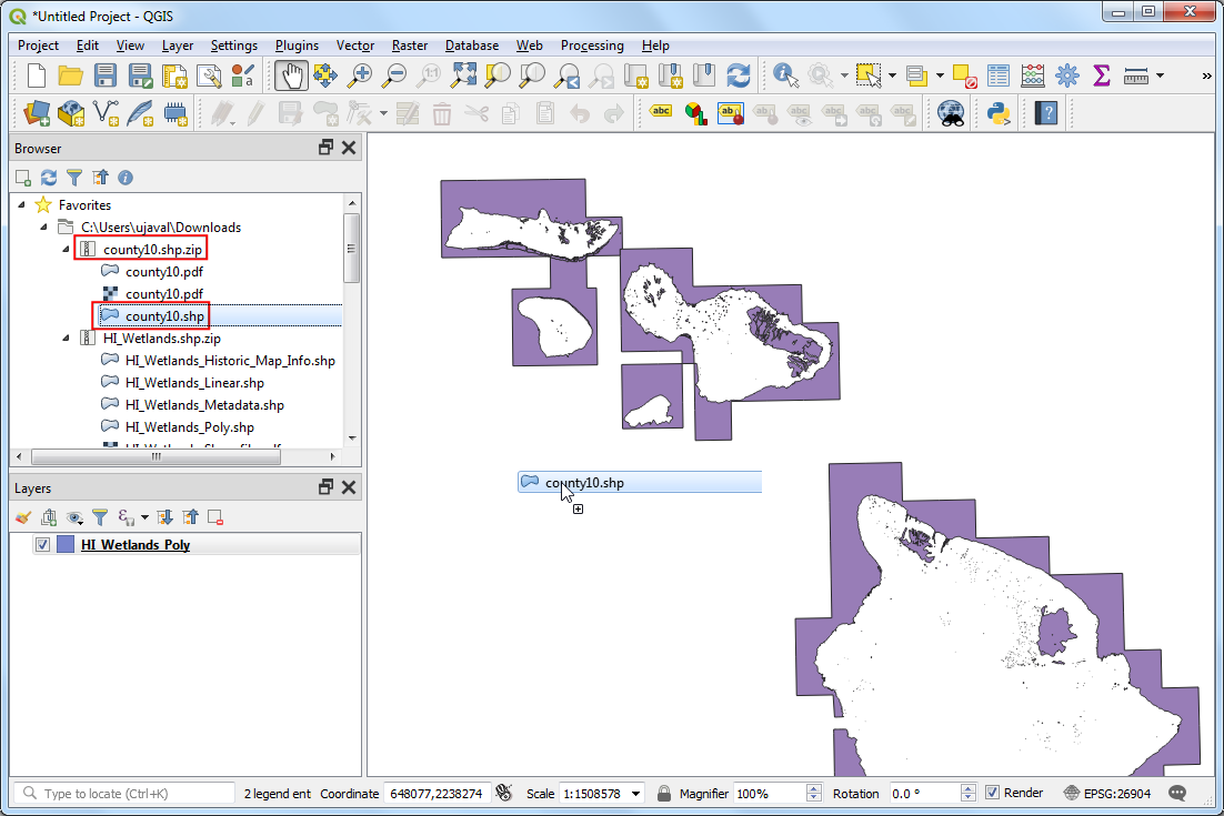
Ker želimo izdelati ločen zemljevid mokrišč za vsako okrožje v državi, bomo potrebovali sloj z mejami okrožij. Poiščite datoteko
county10.shp.zipin jo razširite. Izberite datotekocounty10.shpin jo povlecite na delovno površino.
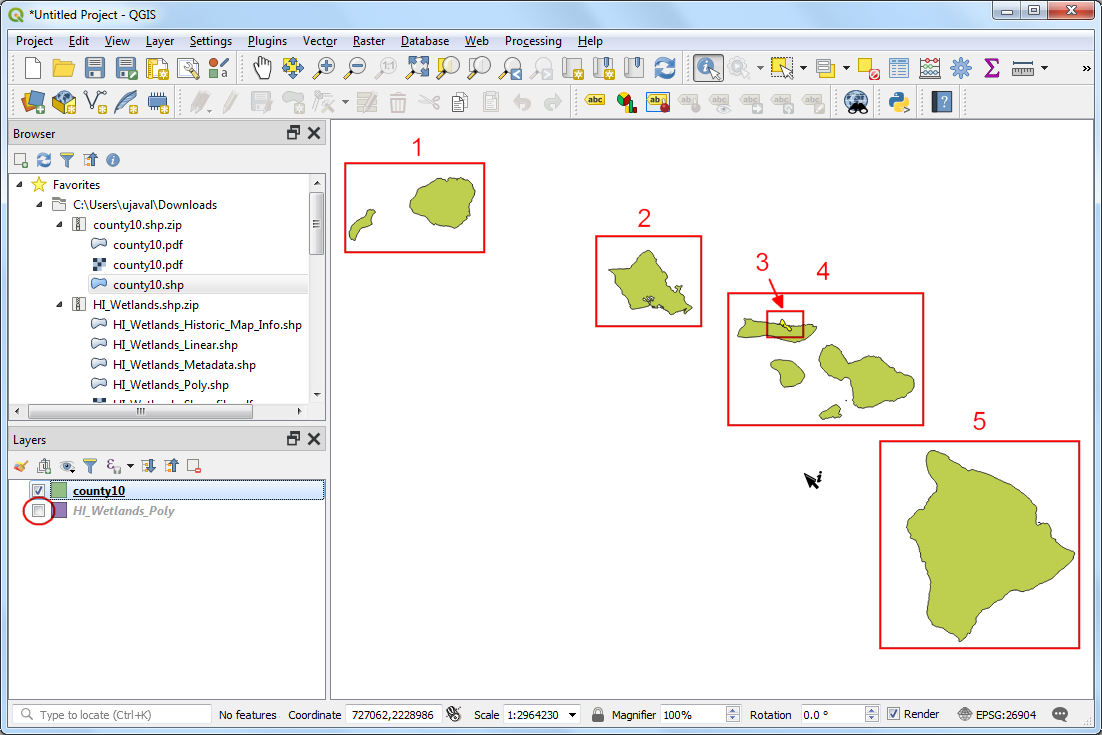
Začasno izklopite vidnost sloja``HI_Wetlands_Poly``. Zdaj boste jasno videli poligone sloja
county10. V tem sloju je 5 elementov, pri čemer je z vsakim elementom povezan 1 ali več poligonov. Značilnosti predstavljajo 5 okrožij. Ta sloj bomo uporabili kot sloj pokritosti in nastavili QGIS, da samodejno ustvari 5 ločenih zemljevidov - enega za vsako značilnost.
Vklopi vidnost sloja``HI_Wetlands_Poly``. Pojdite na .
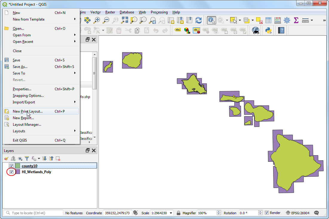
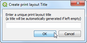
Naslov postavitve tiskanja pustite prazen in kliknite OK.
In the Print Layout window, go to .
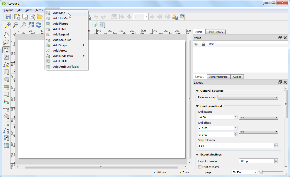
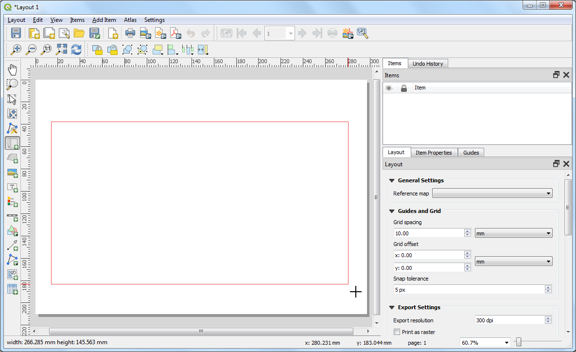
Drag a rectangle while holding the left mouse button where you would like to insert the map.
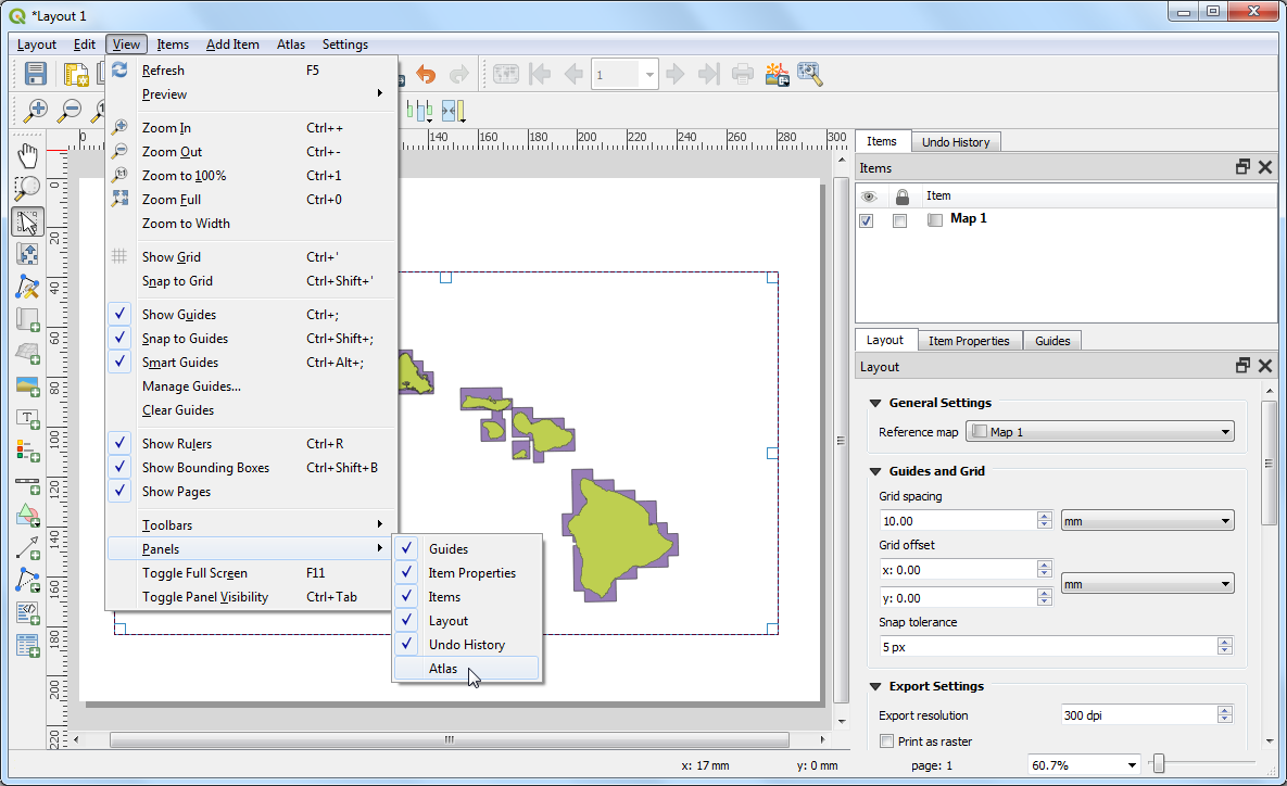
In QGIS3, the Atlas tab is not visible by default. Select .
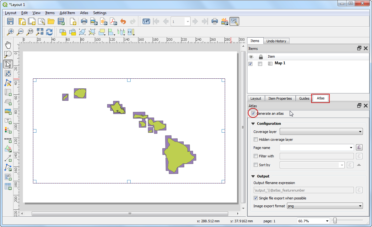
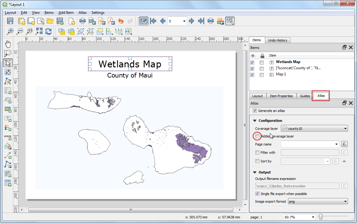
Switch to the Atlas tab. Check the Generate an atlas box.
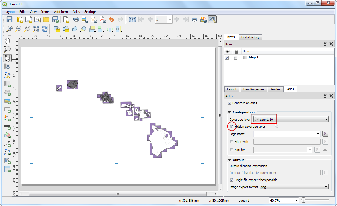
Select the
county10as the Coverage layer. This will indicate that we want to create 1 map each for every polygon feature in thecounty10layer. You can also check the Hidden coverage layer so that the features themselves will not appear on the map.
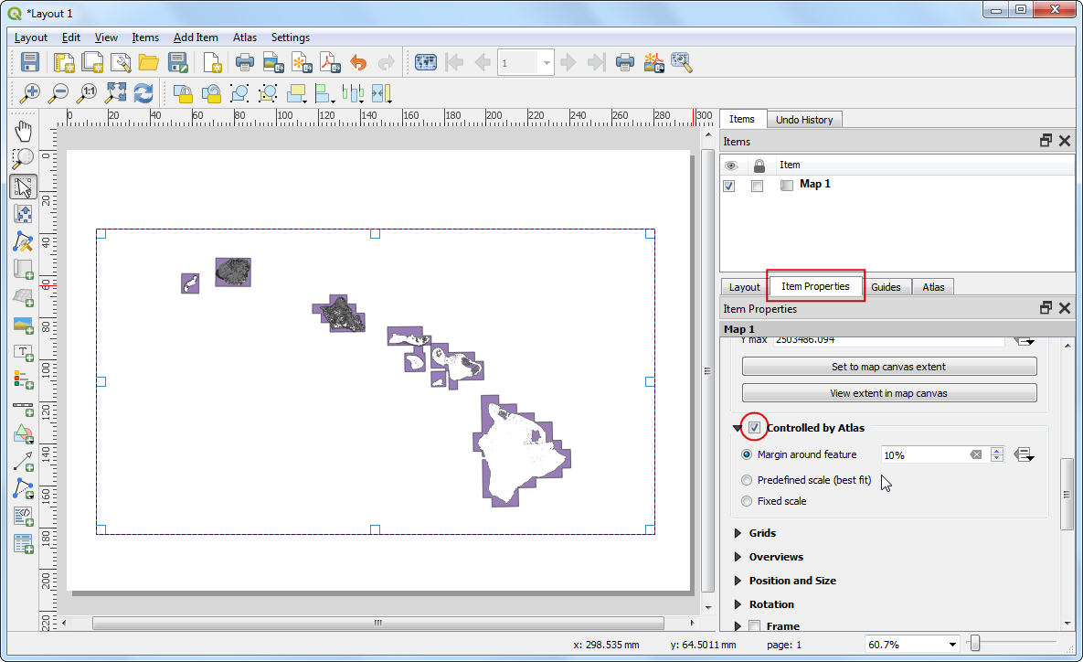
Switch to the Item Properties tab. Scroll down and check the Controlled by atlas box. This will indicate the layout that the content of the map displayed in this item will be determined by the
Atlastool.
Opomba
You must enable the Generare an atlas box in the Atlas tab, otherwise the Controlled by atlas checkbox will be diasbled.
Now that you have configuring the Atlas settings, go to .
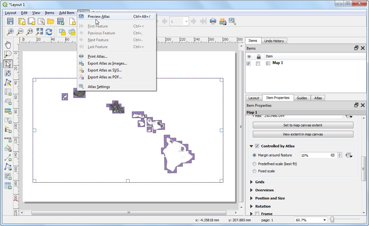
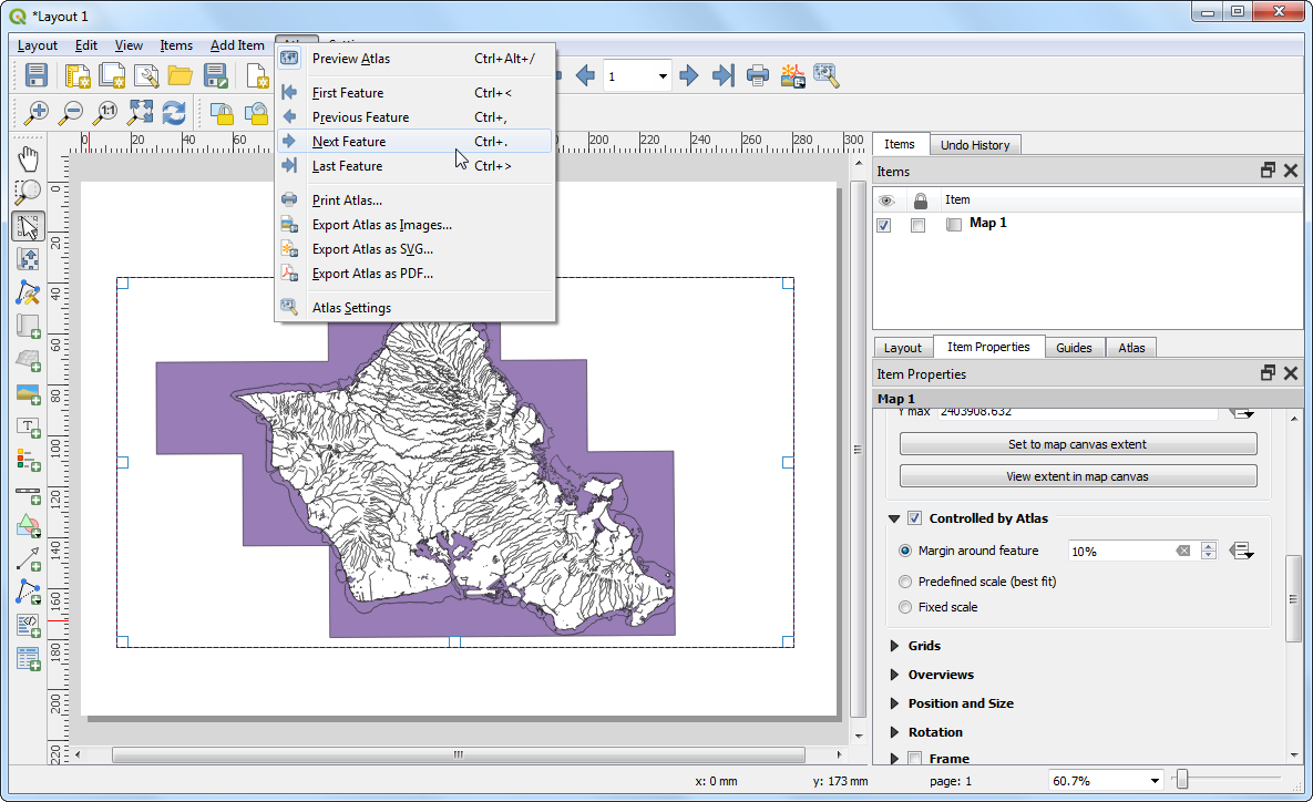
You will see the map refresh and show how individual map will look like. You can preview how the map will look for each of the county polygons. Go to . Atlas will render the map to the extent of the next feature in the coverage layer.
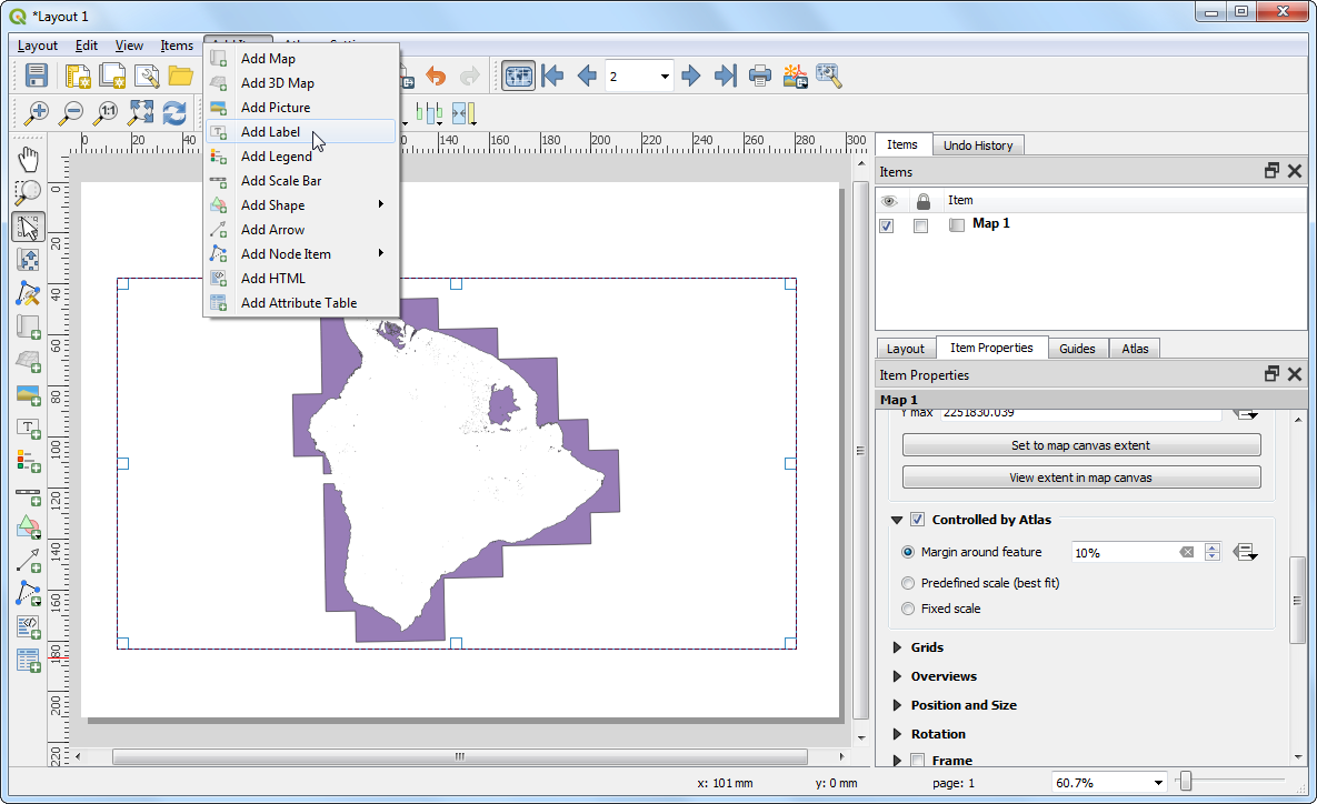
Let’s add a label to the map. Go to .
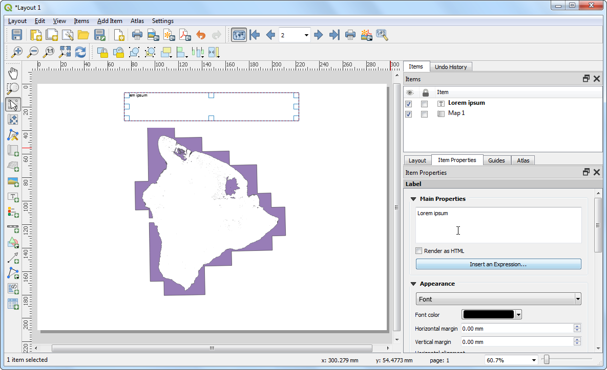
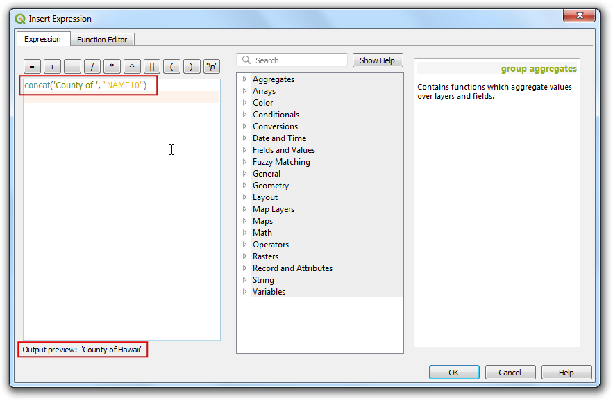
Under the Item properties tab, locate the Main properties section and click Insert an Expression… button.
The label of the map can use the attributes from the coverage layer. The
concatfunction is used to join multiple text items into a single text item. In this case we will join the value of theNAME10attribute of thecounty10layer with the textCounty of. Add an expression like below and click OK.
concat('County of ', "NAME10")
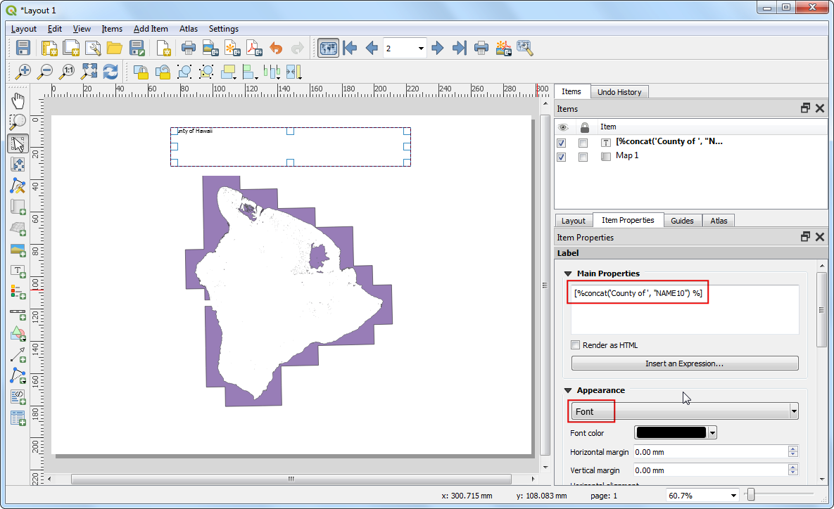
Delete the leading Lorem ipsum placeholder text so that the textbox contains only the expression. Scroll down to the Appearance section and click on the Font dropdown. Choose the font and adjust the size to your liking.
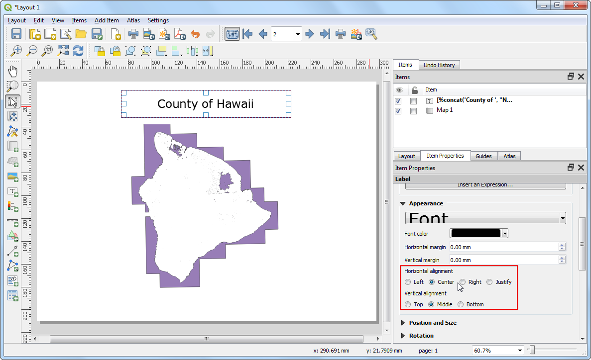
Choose
Centeras the Horizontal alignment andMiddleas the Vertical alignment option.
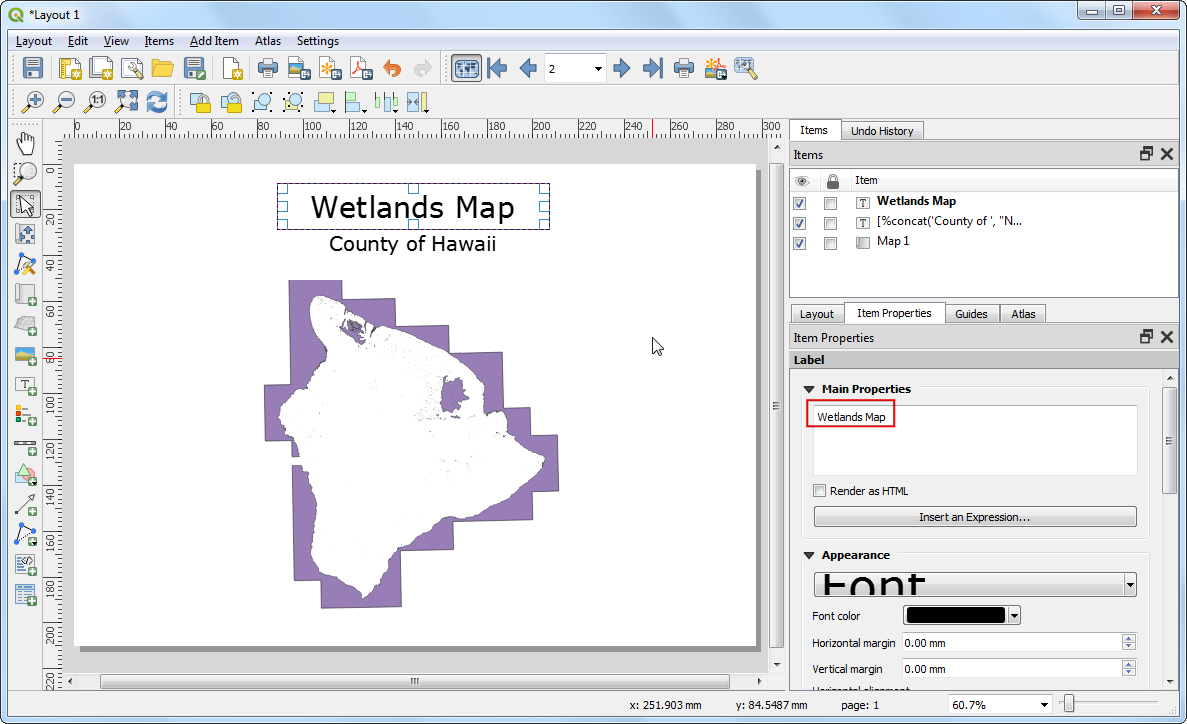
Add another label and enter
Wetlands Mapunder the Main properties. Since there is no expression here, this text will remain the same on all maps.
Go to and verify that the map labels do work as intended. You will notice that the wetland map has polygons extending out in the ocean that looks ugly. We can change the style to that areas outside the county boundaries are hidden.
Switch to the main QGIS window. Right-click the
county10layer and select Properties.
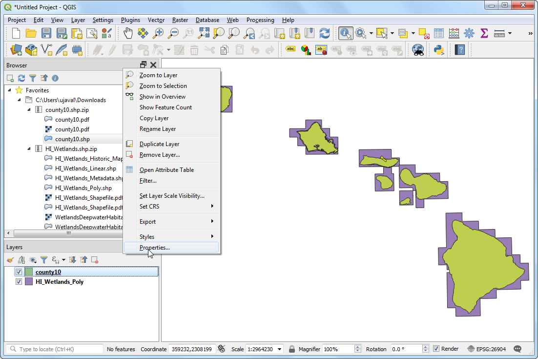
In the Symbology tab, select the Inverted polygons renderer. This renderer styles the outside of the polygon - not inside. Select white as the fill color and click OK.
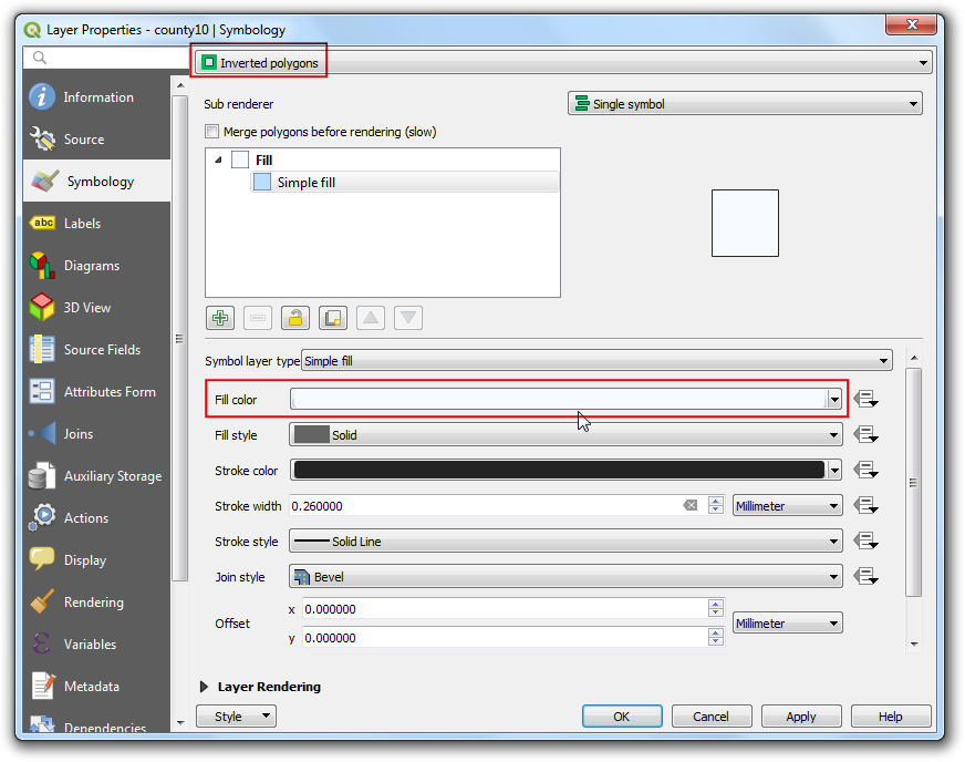
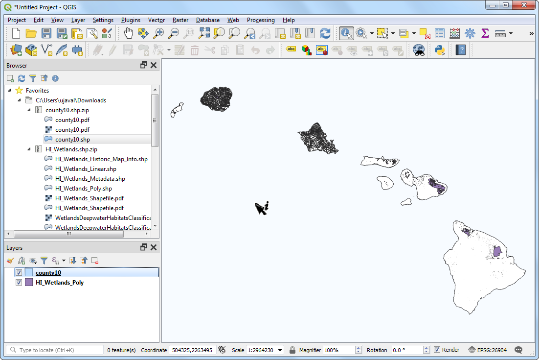
You will notice that the polygons extending outside of the county boundaries are now disappeared. In reality, they are hidden by the white color fill extending out from the county polygons because of the Inverted polygons style.
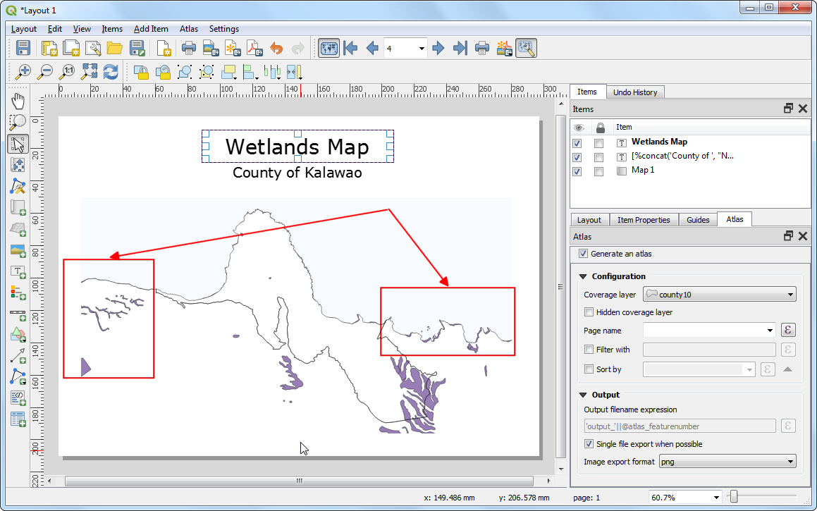
Switch to the Layout window. If we want the effect of the inverted polygons to show, we need to uncheck the Hidden coverage layer box under Atlas tab. Once unchecked, the rendered image will appear clean and areas outside the coverage polygon is not visible.
There is one more problem though. You will notice that in some cases, parts of the map that are outside the coverage layer boundary are still visible. This is because Atlas doesn’t automatically hide other features. This can be useful in some cases, but for our purpose, we only want to show wetlands of the county whose map is being generated. To fix this, switch back to the main QGIS window and right-click the
county10layer and select Properties.
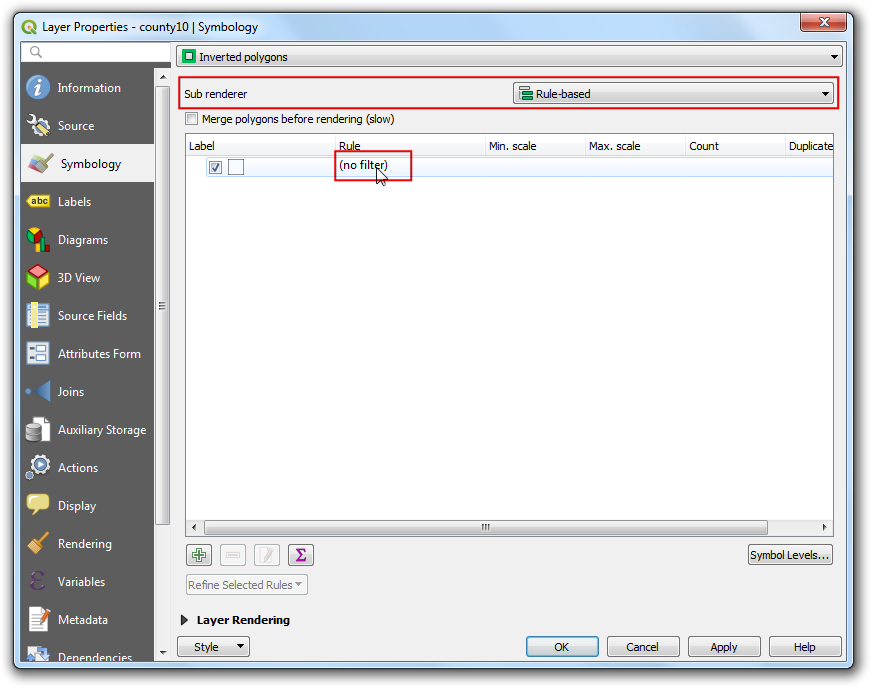
In the Symbology tab, select
Rule-basedas the Sub renderer. Double-click the area under Rule.
In the Edit rule dialog, click the Expression button next to Filter.
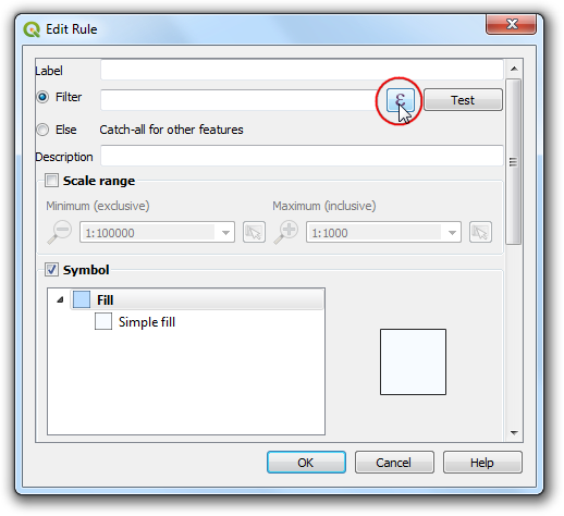
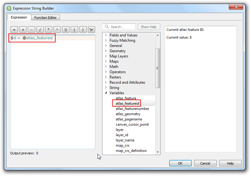
In the Expression string builder, expand the Variables group of functions. The
@atlas_featureidvariable stores the id of the the currently selected feature. We will construct an expression that will select only the currently selected Atlas feature. Enter the expression as below and click OK.
$id = @atlas_featureid
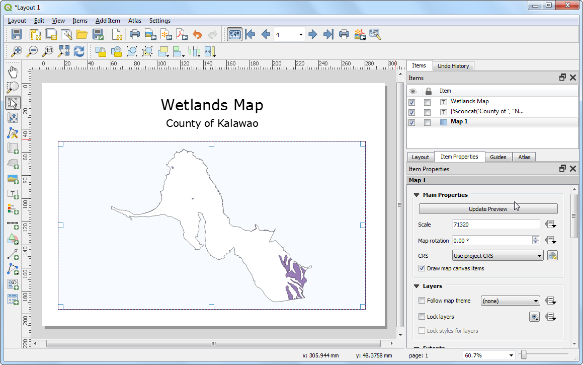
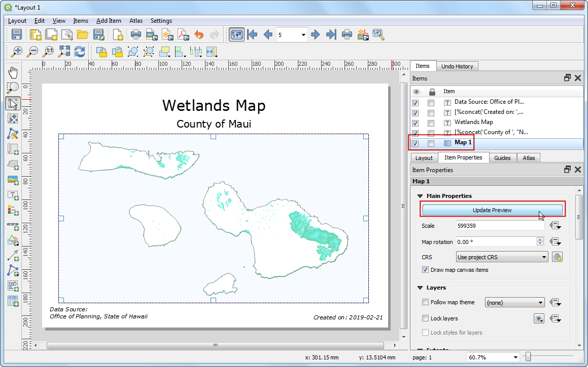
Close all intermediate dialogs and switch back to the Layout window. Select Map 1 item and click the Update preview button under Item properties tab to see the changes. Notice that now only the area covering the county boundary is shown.
Opomba
If you do not see the Update preview button, it may help to select another Item element first and then select Map 1 again.
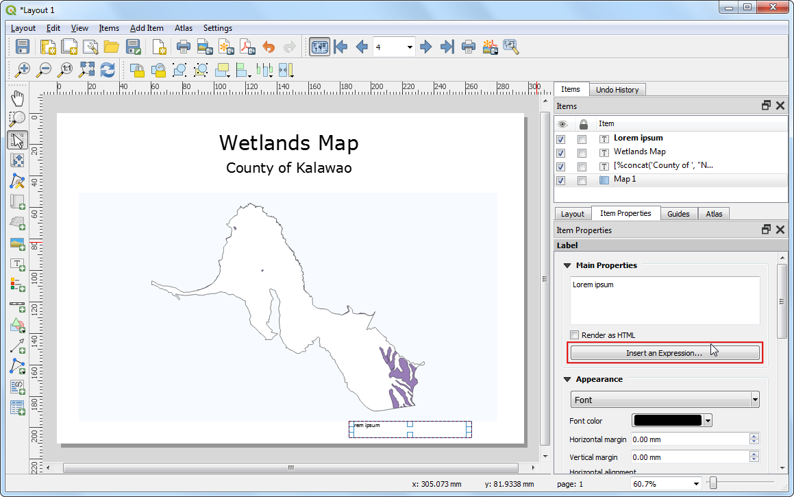
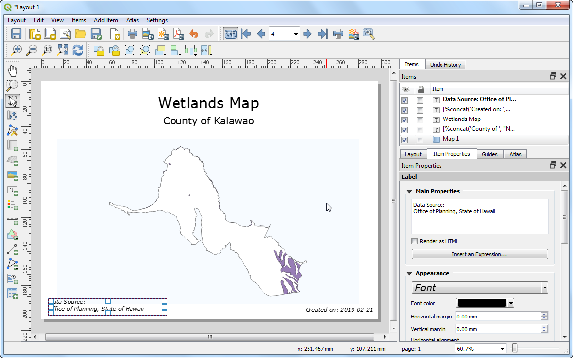
We will now add another dynamic label to show the current date. Go to and select the area on the map. Click Insert an expression button.
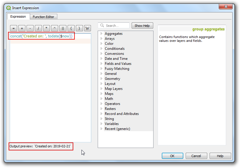
Expand the Date and Time functions group and you will find the
$nowfunction. This holds the current system time. The functiontodate()will convert this to a date string. Enter the expression as below and click OK.
concat('Created on: ', todate($now))
Add another label citing the data source. You may also add other map elements such as a north arrow, scalebar etc. as described in Ustvarjanje karte tutorial.
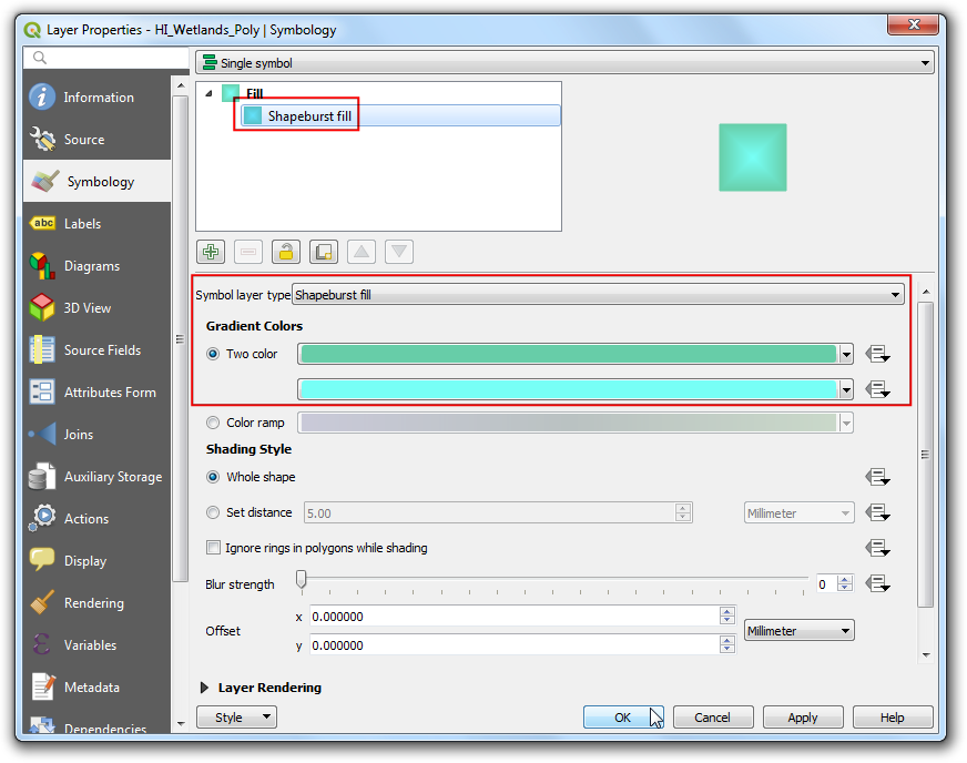
We will make one last styling improvement. Switch back to the main QGIS window and right-click the
HI_Wetlands_Polylayer and select Properties.

In the Symbology tab, click on Simple fill and select
Shapeburst fillas the Symbol layer type. Choose the Two color option and select shades of green and blue that you like. Click OK.
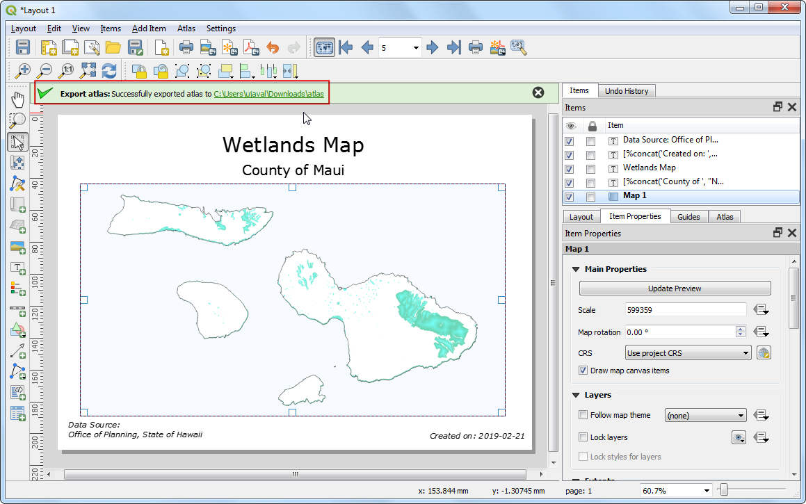
Select Map 1 item and click the Update preview button under Item properties tab to see the changes.
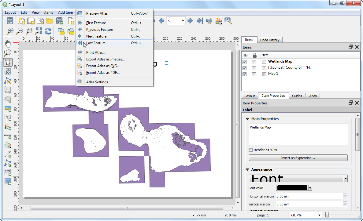
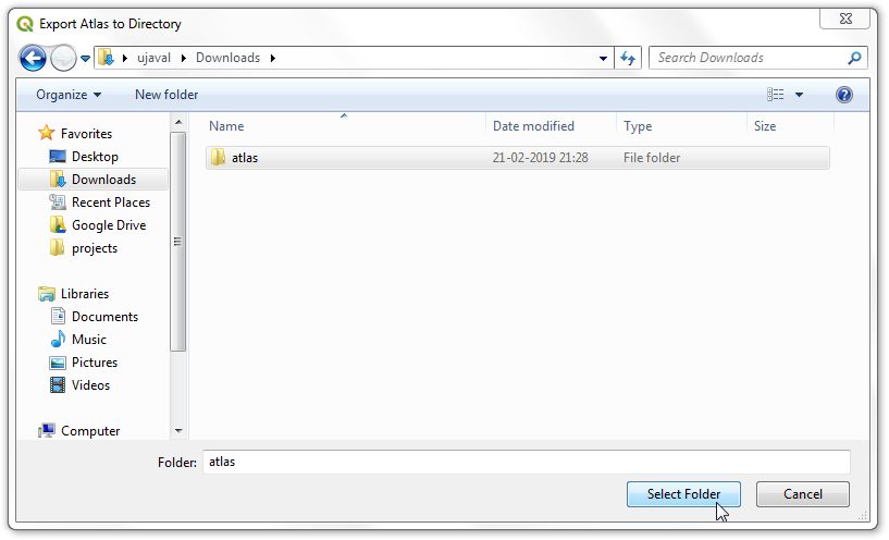
Once you are satisfied with the map layout and styling, go to .
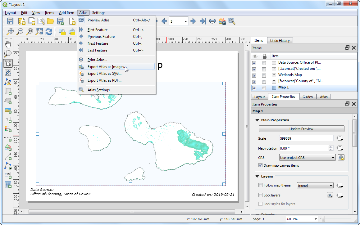
Select a directory on your computer and click Choose.
Leave the default options in the Image Export Options and click Save.
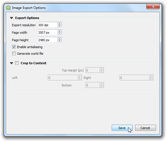
The Atlas tool will now iterate through each feature in the coverage layer and create a separate map image based on the template we created. You can see the images in the directory once the process completes.
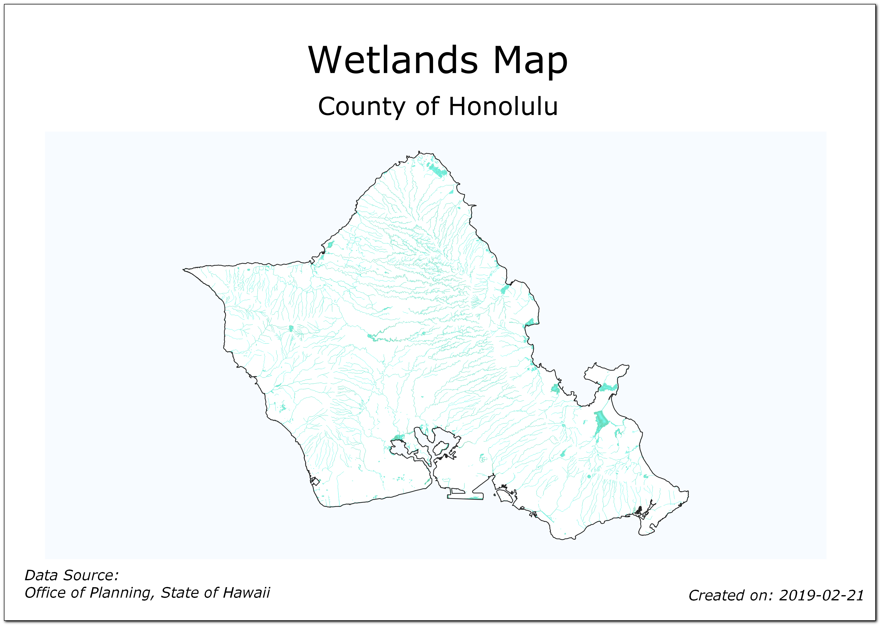
Here are the map images for refeence.
If you want to give feedback or share your experience with this tutorial, please comment below. (requires GitHub account)