 Ujaval Gandhi
Automating Complex Workflows using Processing Modeler (QGIS3)
GIS Workflows typically involve many steps - with each step generating intermediate output that is used by the next step. If you change the input data or want to tweak a parameter, you will need to run through the entire process again manually. Fortunately, QGIS has a graphical modeler built-in that can help you define your workflow and run it with a single invocation. You can also run these workflows as a batch over a large number of inputs.
Overview of the task
We will take a point layer of maritime piracy incidents and create a processing model to produce a density map by aggregating them over a global hexagonal grid.
Other skills you will learn
Using a global equal area projection and setting the Project CRS.
Applying a Graduated symbology to a polygon layer.
Get the data
National Geospatial-Intelligence Agency’s Maritime Safety Information portal provides a shapefile of all incidencts of maritine piracy in the form on Anti-shipping Activity Messages. Download the Arc Shape file version of the database.
Natural Earth has several global vector layers. Download the 10m Physical Vectors - Land containing Land polygons.
For convenience, you may directly download a copy of the above layers from below:
Data Source: [NGA_MSI] [NATURALEARTH]
Procedure
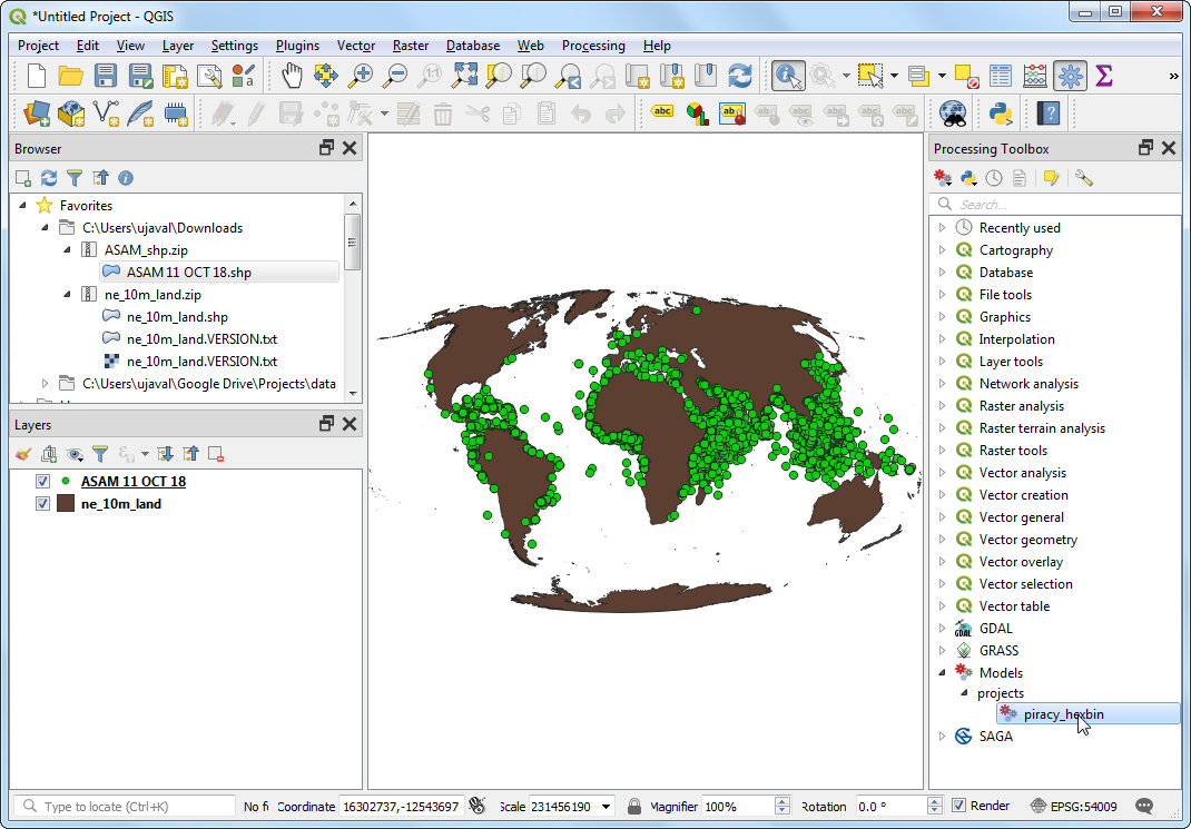
In the QGIS Browser Panel, locate the directory where you saved your downloaded data. Expand the
ne_10m_land.zipand select thene_10m_land.shplayer. Drag the layer to the canvas. Next, locate theASAM_shp.zipfile. Expand it and select theasam_data_download/ASAM_events.shplayer and drag it on to the canvas.
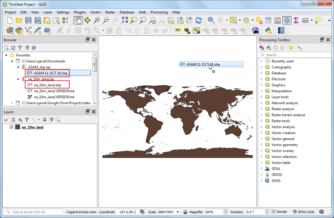
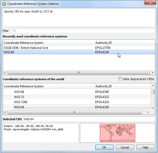
The
ASAM_events.shplayer does not have projection information associated with it, so you will be prompted to select a CRS in the Coordinate Reference System Selector. Here, the points are in the Latitude and Longitude coordinates, so select theWGS 84CRS and click OK.
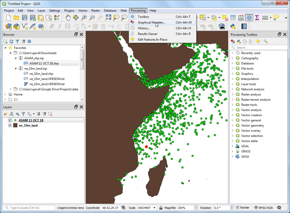
Once the layer is loaded, you can see the individual points representing incidents of piracy locations. Let’s start building our Processing model to process these layers. Go to .
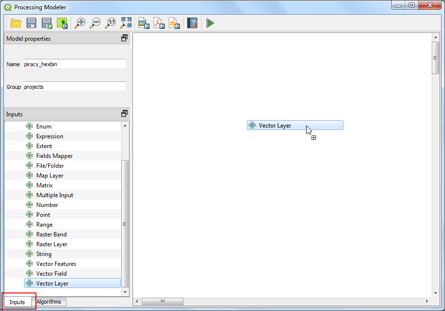
In the Processing Modeler dialog, locate the Model Properties panel. Enter
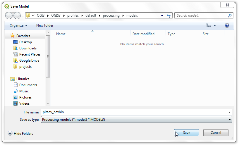
piracy hexbinas the Name of the model andprojectsas the Groups. Click the Save button.
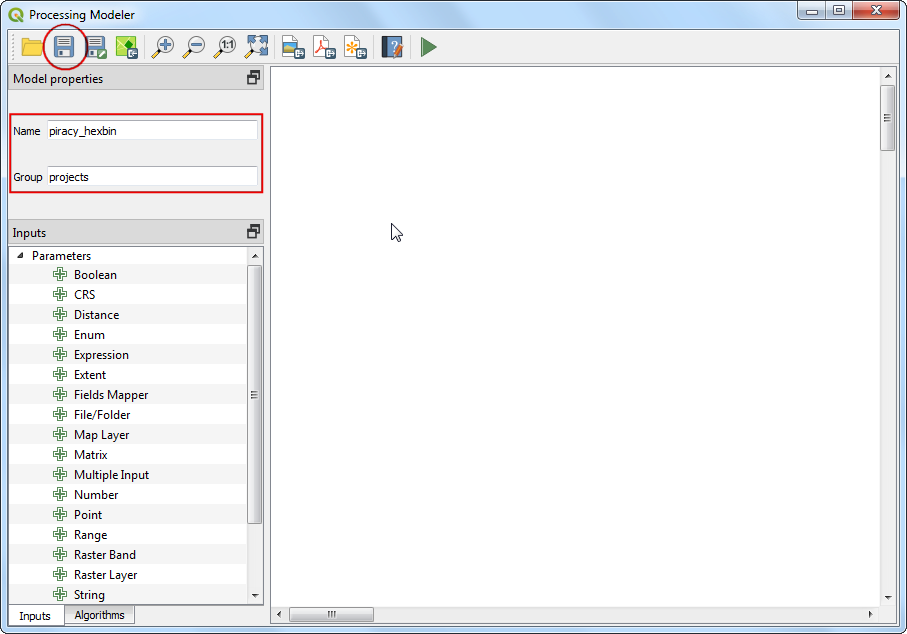
Save the model as
piracy_hexbin.
Now we can start building a graphical model of our processing pipeline. The Processing modeler dialog contains a left-hand panel and a main canvas. On the left-hand panel, locate the Inputs panel listing various types of input data types. Scroll down and select the + Vector Layer input. Drag it to the canvas.
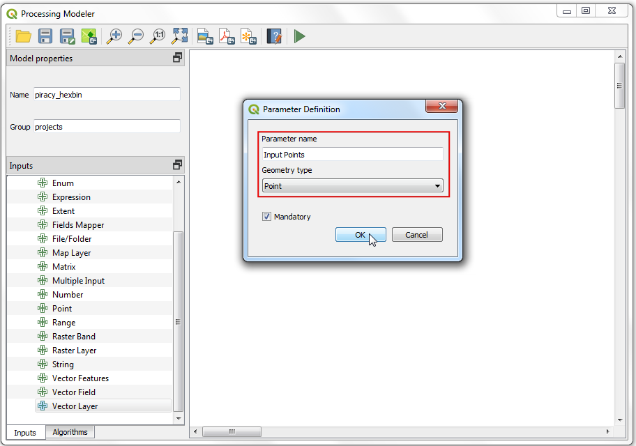
Enter
Input Pointsas the Parameter name andPointas the Geometry type. This input represents the piracy incidents point layer.
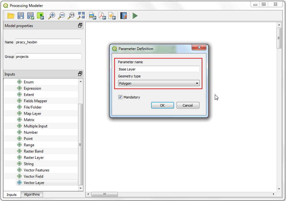
Next, drag another + Vector Layer input to the canvas. Enter
Base Layeras the Parameter name andPolygonas the Geometry type. This input represents the natural earth global land layer.
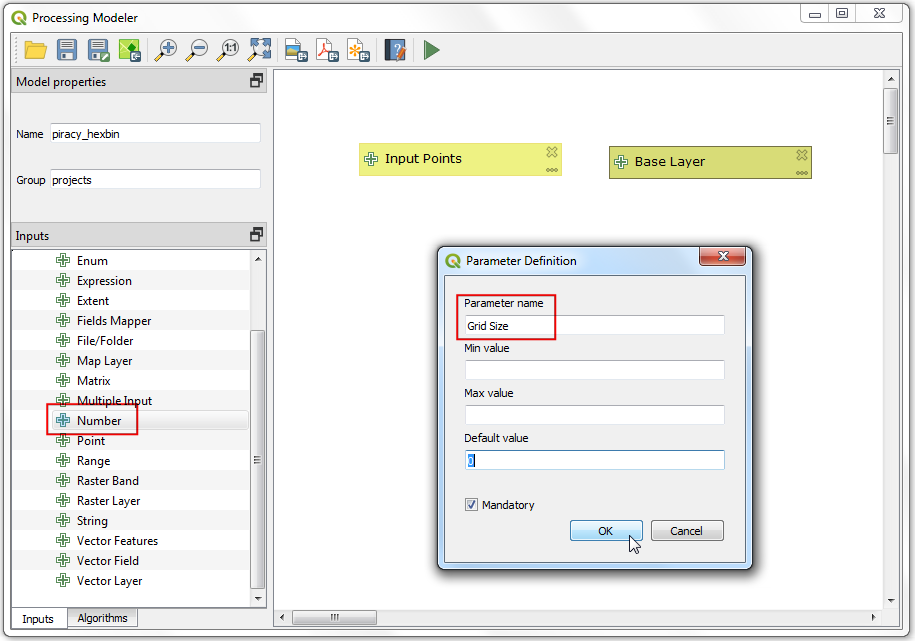
As we are generating a global hexagonal grid, we can ask the user to supply us the grid size as an input instead of hard-coding it as part of our model. This way, the user can quickly experiment with different grid sizes without changing the model at all. select a + Number input and drag it to the canvas. Enter
Grid Sizeas the Parameter name and click OK.
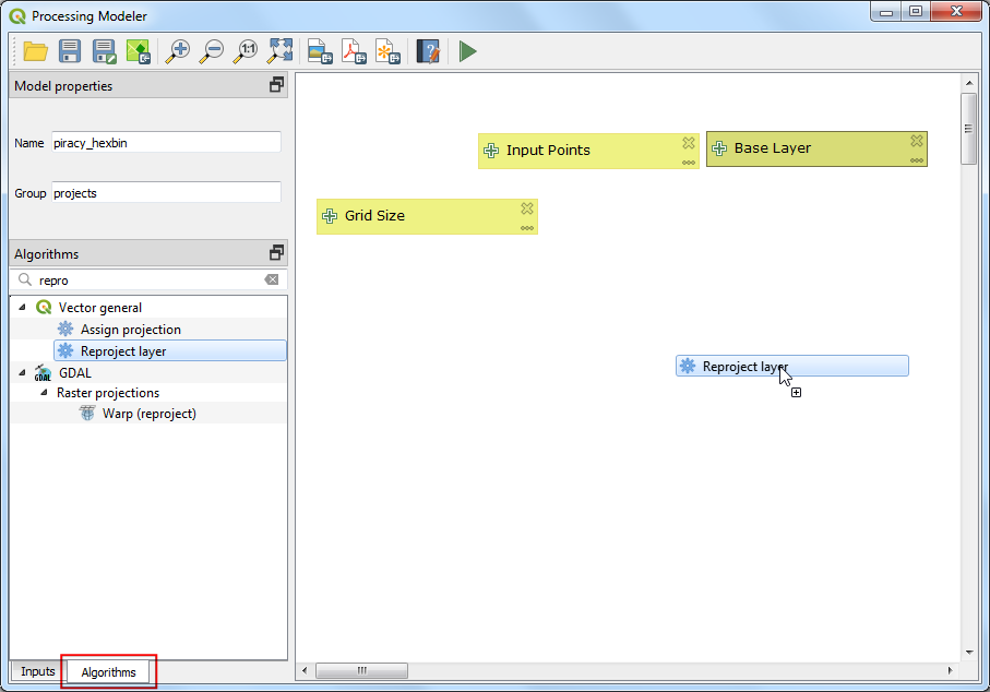
Now that we have our user inputs defined, we are ready to add processing steps. All of the processing algorithms are available to you under the Algorithms tab. The first step in our pipeline will be to reproject the base layer to the Project CRS. Search for
Reproject layeralgorithm and drag it to the canvas.
Note
The necessity of this reprojection step will become clear shortly. The grid generation algorithm requires us to specify the extent of the grid in the unit of the Project CRS. We can supply this reprojected layer to compute this extent.
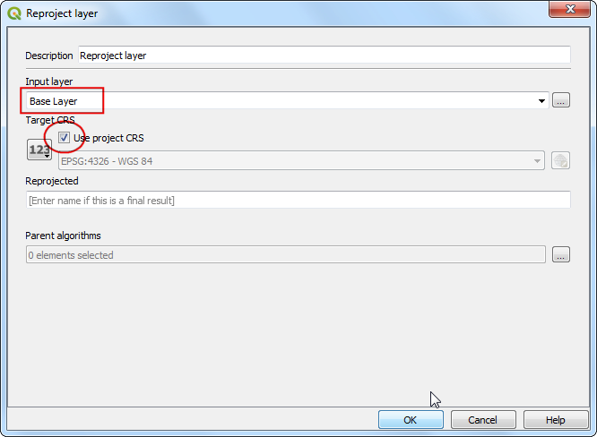
In the Reproject layer dialog, select
Base Layeras the Input layer. Check the Use project CRS as the Target CRS. Click OK.
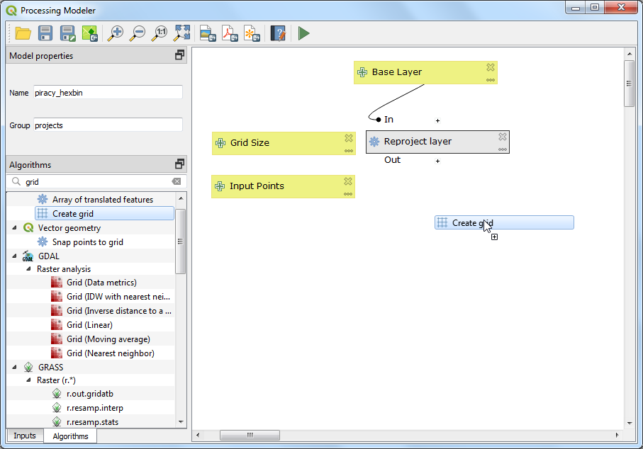
In the Processing Modeler canvas, you will notice a connection appear between the + Base Layer input and the Reproject layer algorithm. This connection indicates the flow of our processing pipeline. Next step is to create a hexagonal grid. Search for the
Create gridalgorithm and drag it to the canvas.
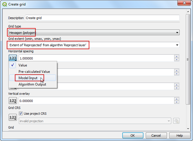
In the Generate grid dialog, choose
Hexagon (polygon)as the Grid type. SelectExtent of 'Reprojected' from algorithm 'Reproject Layer'as the Grid extent. Click the 123 button under the Horizonal spacing label and choose Model input.
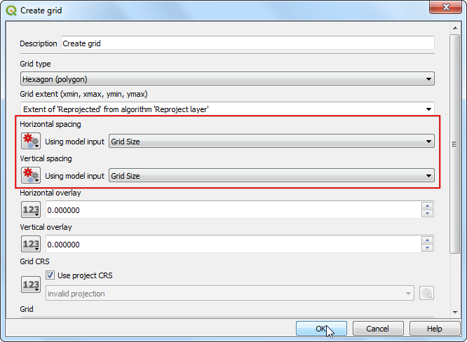
Select
Grid Sizeinput for Using model input. Repeat the same process for Vertical Spacing. Click OK.
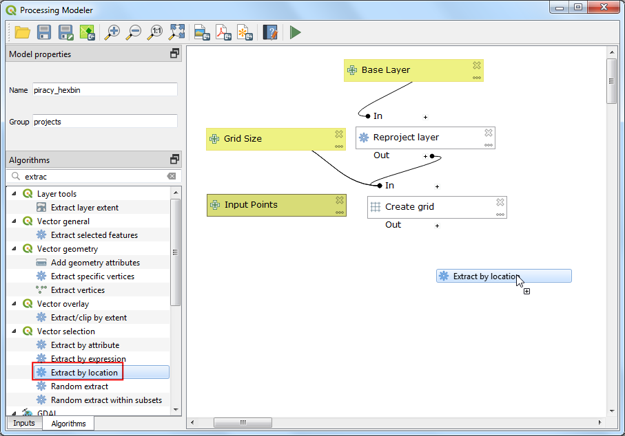
At this point, we have a global hexagonal grid. The grid spans the full extent of the base layer, including land areas and places where there are no points. Let’s filter out those grid polygons where there are no input points. Search for
Extract by locationalgorithm and drag it to the canvas.
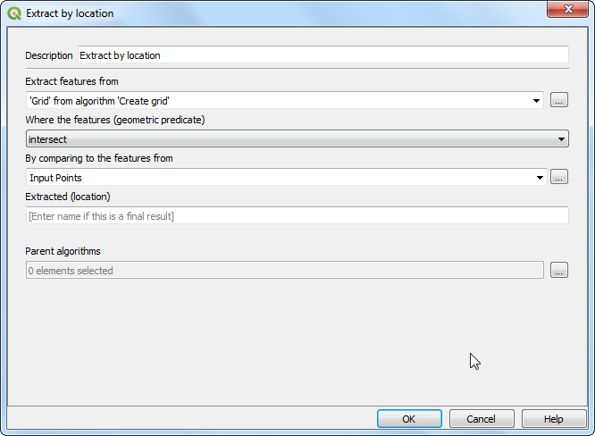
For Extract features from, select
'Grid' from algorithm 'Generate Grid', Where the features (geometric predicate) asIntersectand By comparing to the features from asInput points. Click OK.
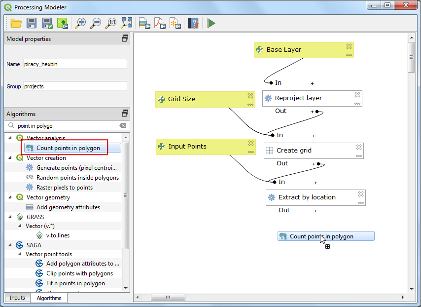
Now we have only those grid polygons that contain some input points. To aggregate these points, we will use
Count points in polygonalgorithm. Search and drag it to the canvas.
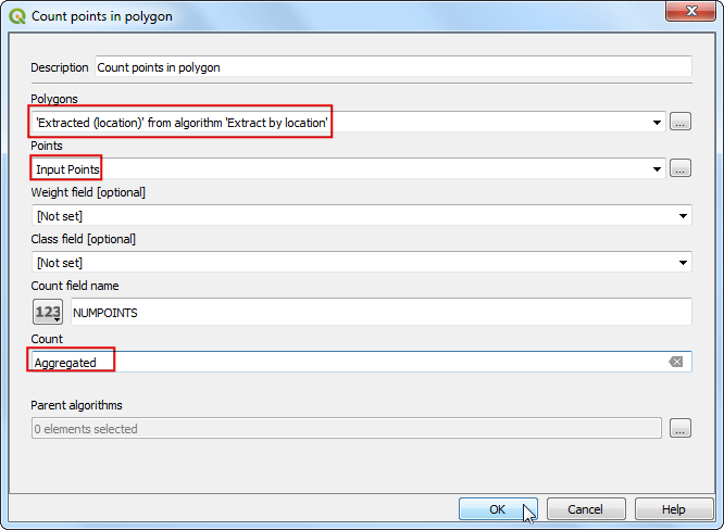
Select
'Extracted (location)' from algorithm 'Extract by location'as the value for Polygons. The Points layer would beInput Points. At the bottom, name the Count output layer asAggregated. Click OK.
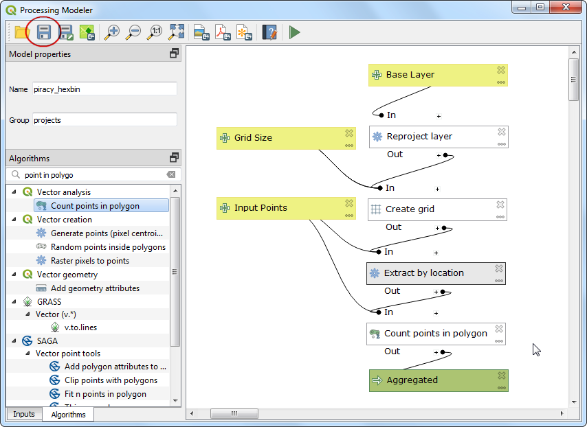
The model is now complete. Click the Save button.
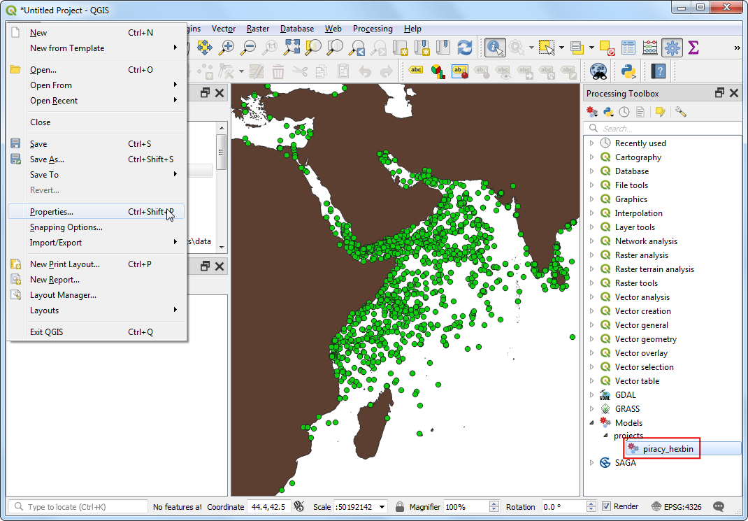
Switch to the main QGIS window. You can find your newly created model in the Processing Toolbox under . Now it is time to run and test the model. As our goal is to aggregate the input points over hexagonal grids, it is important that the grids are generated using a equal-area projection. This will ensure that regardless of the location of the grid, it will cover exactly the same area. Our model doesn’t explicitely ask for a CRS, but uses whatever CRS is set as the Project CRS. Let’s choose a global equal area projection as the Project CRS. Go to .
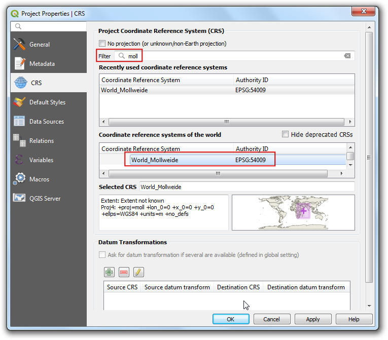
In the Project Properties dialog, switch to the CRS tab. We will use a global Mollweide projection for this exercise which is a equal area projection. Search for
Mollweidein the Filter box and selectWorld_Mollweide EPSG:54009as the CRS. Click OK.
You will see the layers getting reprojected on-the-fly to the selected CRS. Locate the
piracy_hexbinmodel in the Processing Toolbox and double-click it.
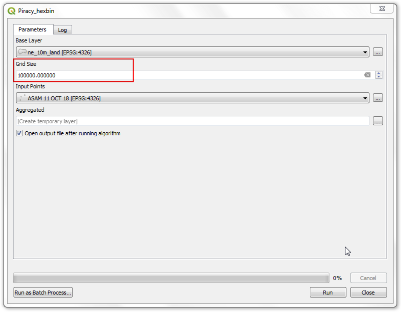
Our Base Layer is the
ne_10m_landand the Input Points layer isASAM_events. The Grid Size needs to be specified in the units of the selected CRS. The World_Mollweide CRS unit is meters, so we specify100000m (100 Kms) as the Grid Size. Click Run to start the processing pipeline. Once the process finishes, click Close.
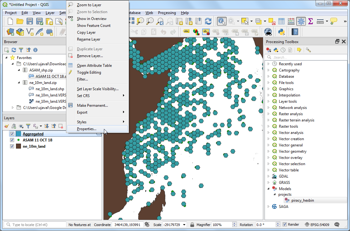
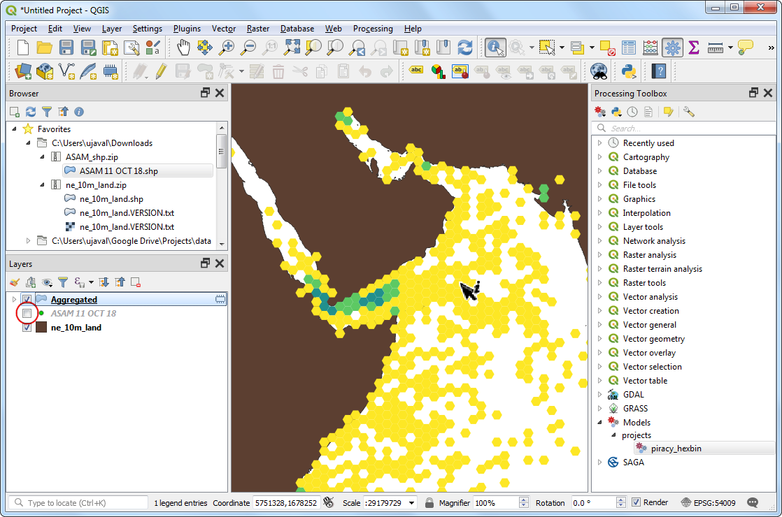
You will see a new layer
Aggregatedloaded as the result of the model. As you explore, you will notice the layer contains an attribute called NUMPOINTS containing the number of piracy incidents points contained within that grid feature. Let’s style this layer to display this information better. Right-click theAggregatedlayer and select Properties.
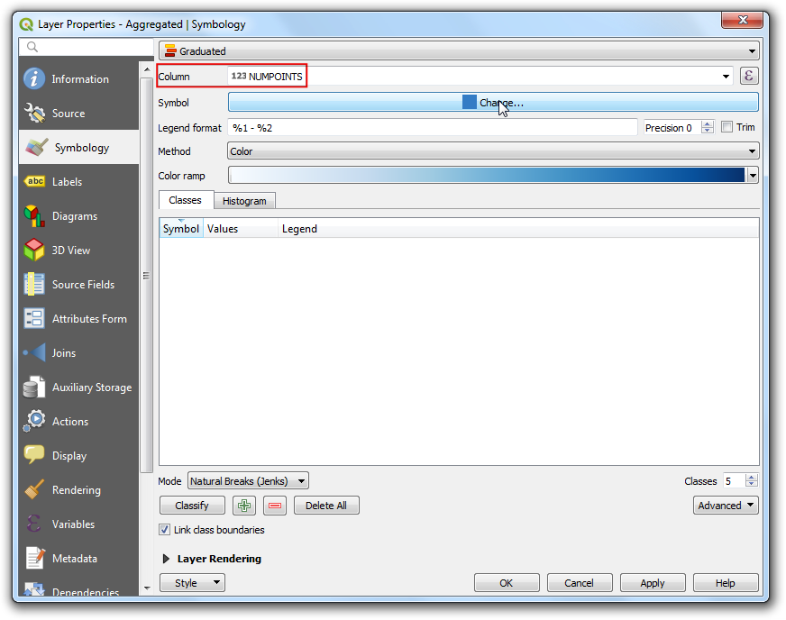
Switch to the Symbology tab. Select
Graduatedsymbology andNUMPOINTSas the Column. ClickChange..next to Symbol label.
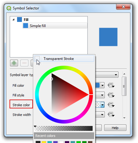
Select Simple fill symbol and check the Transparent Stroke button under Stroke color. This is to make the hexagon edges transparent.
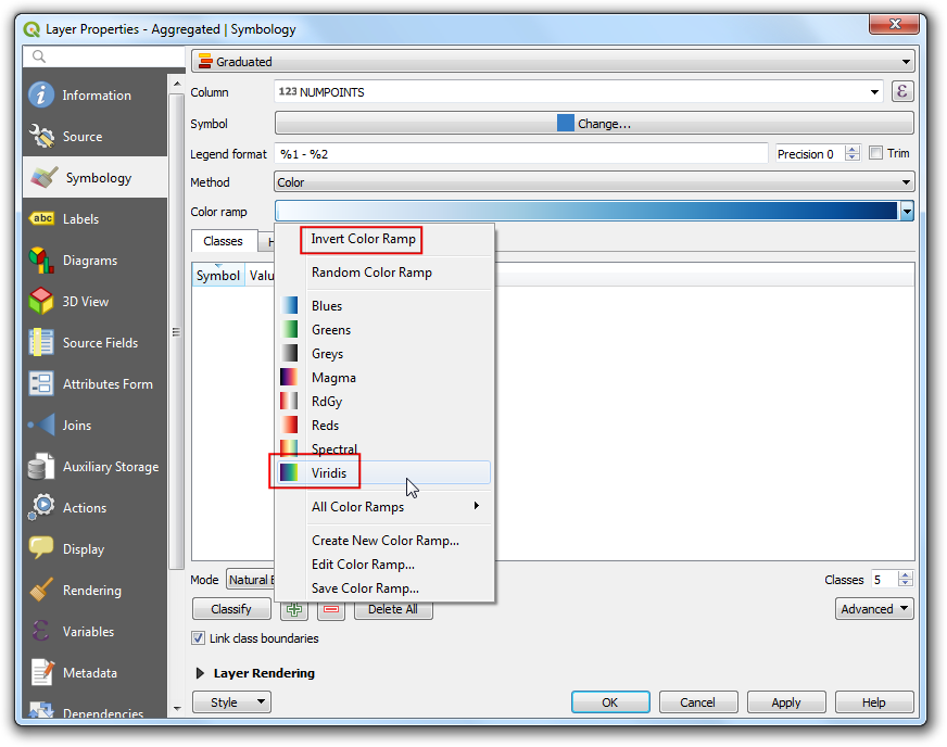
Click the dropdown next to Color ramp and select the
Viridisramp. Click the dropdown again and select Invert Color Ramp to reverse the order of color.
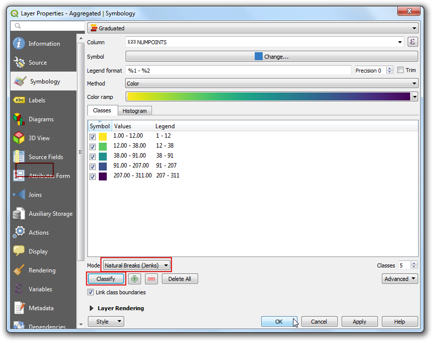
The Graduated symbology will divide the values in the selected column into distinct classes and assign a different color to each of the classes. Select
Natural Breaks (Jenks)as the Mode and click Classify and click OK.
Note
see Basic Vector Styling for a detailed explanation of different modes.
Back in the main QGIS window, turn off the
ASAM_eventslayer. You will see a nice visualization of piracy hotspots across the globe.
Now that you have encoded the full data pipeline in the model, it is easy to reproduce your results. A model also allows you to experiment quickly without manually repeating each intermediate step every time. If your inputs change over time, say an updated database of piracy is released after a few months, you can run your model on that input to generate a similar visualization without having to remember each step.
If you want to give feedback or share your experience with this tutorial, please comment below. (requires GitHub account)