Multikriterielle Überlagerungs-Analyse (QGIS3)

Unter gewichteter multikriterieller Überlagerungs-Analyse wird die Auswahl von Flächen auf der Basis mehrerer Attribute verstanden, die im Untersuchungsgebiet definiert sein sollten. Obwohl es sich um eine verbreitete GIS-Technik handelt, wird diese am effizientesten mit einem gitterbasierten Ansatz auf Rasterdaten ausgeführt.

Bemerkung

Vektor- vs. Raster-Überlagerungen

You can do the overlay analysis on vector layers using geoprocessing tools such as buffer, dissolve, difference and intersection. This method is ideal if you wanted to find a binary suitable/non-suitable answer and you are working with a handful of layers. You can review our video tutorial on Locating A New Bicycle Parking Station using Multicriteria Overlay Analysis for a step-by-step guide on this approach.

Die Arbeit mit Rasterdaten ergibt eine Rangfolge der Eignung und nicht nur die am besten geeignete Fläche. Sie ermöglicht es auch, einfach eine beliebige Anzahl an Eingabelayern zu kombinieren und jedem verwendeten Kriterium eine unterschiedliche Wichtung zuzuweisen. Es handelt sich um das allgemein bevorzugte Vorgehen für die Bewertung der Eignung von Flächen.

Dieses Tutorial behandelt den typischen Arbeitsablauf für die Ausführung einer Flächeneignungsanalyse. Es werden Vektor-Quelldaten zu geeigneten Rasterdaten konvertiert. Letztere werden re-klassifiziert und mathematischen Operationen unterzogen.

Überblick über die Aufgabe

In diesem Tutorial bestimmen wir geeignete Flächen für die Erschließung, welche sich

• nah an Straßen und

• abseits von Gewässern und

• nicht in Schutzgebieten befinden.

Beschaffung der Daten

Wir verwenden Layer von Vektordaten aus dem OpenStreetMap-Projekt (OSM). OSM ist eine Datenbank weltweit frei verfügbarer Basis-Kartendaten. Geofabrik vertreibt täglich aktualisierte Shapefiles der OpenStreetMap-Datensätze.

We will be using the OSM data layers for the state of Assam in India. Geofabrik India shapefiles were downloaded, reprojected to a UTM projection, clipped to the state boundary and packaged in a single GeoPackage file. You can download a copy of the geopackage from the link below:

assam.gpkg

Datenquelle: [GEOFABRIK]

Arbeitsablauf

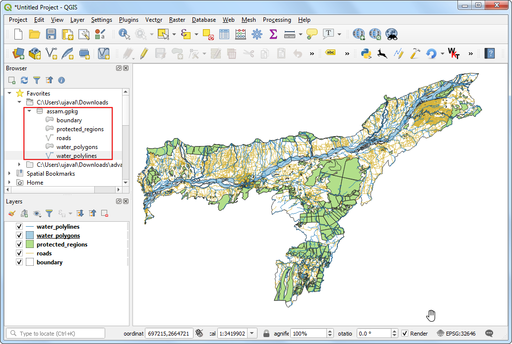
1. Wir suchen die heruntergeladene Datei assam.gpkg im QGIS-Browser, erweitern sie und ziehen jeden der 5 Datenlayer in den Arbeitsbereich. Die Layer boundary, roads, protected_regions, water_polygons und water_polylines werden in das Layer-Panel geladen.

2. Der erste Schritt der Überlagerungs-Analyse besteht darin, jeden der Datenalyer in einen Rasterlayer zu konvertieren. Es ist wichtig, dass alle entstehenden Rasterlayer dieselbe Ausdehnung haben. Wir verwenden den boundary-Layer als Begrenzung für die Rasterlayer. wir wählen Verarbeitung ‣ Werkzeugkiste und suchen den Algorithmus GDAL ‣ Vektorkonvertierung ‣ Rastern (Vektor nach Raster) und starten ihn per Doppelklick.

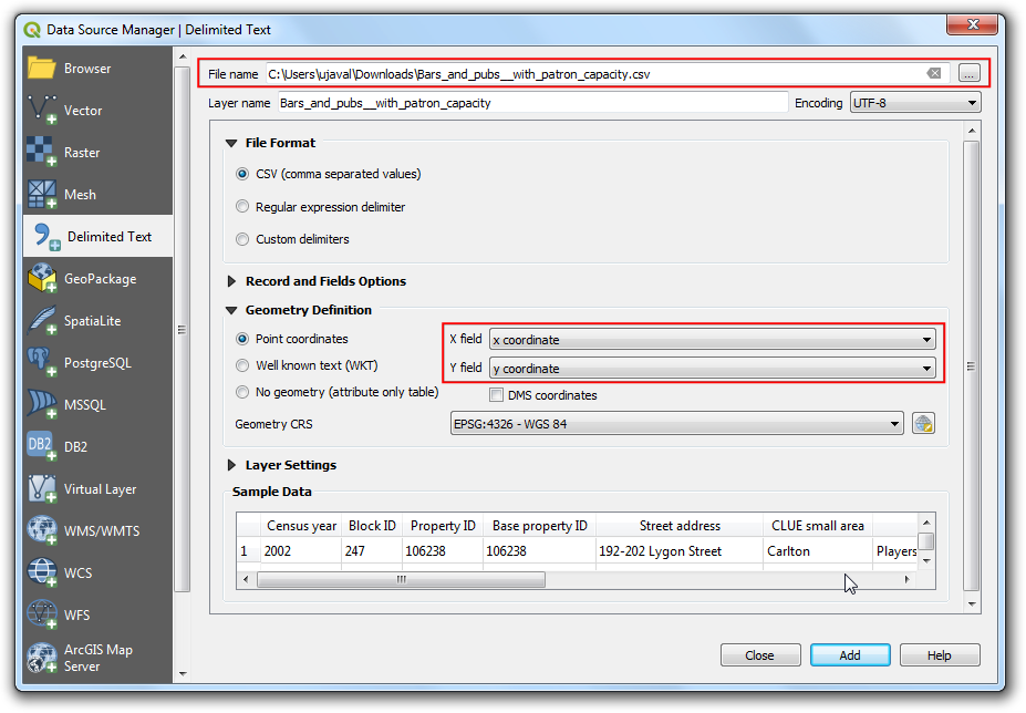
3. In the Vector Conversion - Rasterize (vector to raster) dialog, select roads as the Input layer. We want to create an output raster where pixel values are 1 where there is a road and 0 where there are no roads. Enter 1 as the A fixed value to burn. The input layers are in a projected CRS with meters are the unit. Select Geoferenced units as the Output raster size units. We will set the resolution of the output raster to be 15 meters. Select 15 as both Width/Horizontal resolution and Height/Vertical resolution. Next, click the arrow next to Output extent and select Calculate from Layer ‣ boundary.

4. Im Abschnitt Fortgeschrittene Parameter weiter unten wählen wir als Profil Hohe Kompression, um das Bild zu komprimieren. Das komprimierte Rasterbild wird dadurch nach Anwenden des Werkzeugs weniger Speicherplatz beanspruchen. Eine verlustlose Kompression ist für die Arbeit mit Rasterdatan dringend zu empfehlen.

5. Unter Gerastert -> In Datei speichern… geben wir raster_roads.tif als Ausgaberaster an und betätigen die Schaltfläche Starte.

6. Once the processing finishes, you will see a new layer raster_roads loaded in the Layers panel. The raster has pixel values 1 for pixels which intersected with the roads. All other pixels are set as NoData values. These nodata values are problematic because when raster calculator (which we will use later) encounters a pixel with nodata value in any layer, it sets the output value of that pixel to nodata as well, resulting is unexpected output. We will fill these nodata values with the value 0. Search for and locate the Raster Tools ‣ Fill NoData cells algorithm. Double-click to launch it.

7. Select raster_roads as the Raster input and choose 0 as the Fill value. Scroll down to find the Advanced Parameters and select the profile High Compression to apply the compression. Set the Output raster as raster_roads_filled.tif and click Run.

8. Once the processing finishes, you will see the new layer raster_roads_filled loaded in the Layers panel. This raster has values 1 for roads and 0 for no roads. If the layer is not visualized correctly, you can click the Open the Layer Styling Panel and set the Min to 0 and Max to 1.

9. Repeat steps 3-8 for the other 3 vector layers protected_regions, water_polylines and water_polygons layers. You need to rasterize and fill the nodata cells for these layers. If you want to run these steps manually, you can configure the processing algorithm dialog, run the algorithm and once the algorithm finishes, switch to the Parameters tab and just change the input and output layer names. You can also run each algorithm on all 4 layers in a single step using Batch Processing. See the Stapelverarbeitung mit dem Processing Framework (QGIS3) tutorial to learn more. Once you are done, you should have 4 raster layers and generate the corresponding raster layers raster_roads_filled, raster_protected_regions_filled, raster_water_polylines_filled and raster_water_polygons_filled. You will notice that we have 2 water related layers - both representing water. We can merge them to have a single layer representing water areas in the region. Search for and locate Raster analysis ‣ Raster calculator algorithm in the Processing Toolbox. Double-click to launch it.

10. Select raster_water_polygons and raster_water_polylines layers using … button as Input Layers. Enter the following expression using ε button. Keep all the other options as default and save the output layer with the name raster_water_merged.tif and click Run.

"raster_water_polygons_filled@1" + "raster_water_polylines_filled@1"

11. Das Ergebnis enthält Pixel mit dem Wert 1 für alle Gebiete mit Wasserflächen. Es gibt jedoch auch einige Regionen, in denen sowohl Wasser-Polygone als auch -Linien verzeichnet sind. Dort werden sich Pixel mit dem Wert 2 finden lassen ‒ was nicht korrekt ist. Wir können dies aber mit einem einfachen Ausdruck beheben. Wir wählen den Rasteranalyse ‣ Rasterrechner erneut.

12. Select raster_water_merged layer using … button as an Input Layer. Enter the following expression using ε button. Keep all the other options as default and save the output layer with the name raster_water_filled.tif and click Run.

"raster_water_merged@1" > 0

13. The resulting layer raster_water_filled now has pixels with only 0 and 1 values.

14. Mithilfe der Layer für Straßen und Gewässer können wir nun Nachbarschaftsraster erstellen. Diese werden auch Euklidische Distanzen genannt, bei denen jeder Pixel im Ausgaberaster den Abstand zum nächstgelegenen Pixel im Eingaberaster repräsentiert. Das Ergebnisraster kann anschließend verwendet werden, um geeignete Gebiete innerhalb eines bestimmten Abstandes von den Eingabepixeln zu definieren. Wir suchen den Algorithmus GDAL ‣ Rasteranalyse ‣ Nähe (Rasterabstand) und starten ihn per Doppelklick.

15. In the Raster Analysis - Proximity (Raster Distance) dialog, select raster_roads_filled as the Input layer. Choose Georeferenced coordinates as the Distance units. As the input layers are in a projected CRS with meters as the units, enter 5000 (5 kilometers) as the Maximum distance to be generated. For all pixels that are more than the maximum distance away - we will set their values to be 5000 as well. So set the Nodata value to use for the destination proximity raster value to 5000.

16. Nach Erweiterung des Bereichs Fortgeschrittene Parameter wählen wir als Profil Hohe Kompression aus. Die Ausgabedatei benennen wir mit roads_proximity.tif und betätigen die Schaltfläche Starte.

Bemerkung

It may take upto 15 minutes for this process to run. It is a computationally intensive algorithm that needs to compute distance for each pixel of the input raster.

17. Nach Abschluss der Berechnungen wird ein neuer Layer roads_proximity zum Layer-Panel hinzugefügt. Um ihn besser zu visualisieren, sollten wir die Voreinstellung für die Darstellung ändern. Wir betätigen die Schaltfläche Layergestaltungsfenster öffnen im Layer-Panel und ändern den Max-Wert unter Farbverlauf auf 5000.

18. Repeat the Proximity (Raster Distance) algorithm for the raster_water_filled layer with same parameters and name the output water_proximity.tif. If you click around the resulting raster, you will see that it is a continuum of values from 0 to 5000. To use this raster in overlay analysis ,we must first re-classify it to create discrete values. Open Raster analysis ‣ Raster calculator algorithm again.

19. Auf näher an der Straße gelegene Pixel wollen wir höhere Bewertungen anwenden; dazu benutzen wir das folgende Schema.

• 0 - 1000 m –> 100

• 1000-2000m –> 50

• >2000m –> 10

  Select roads_proximity layer using … button as an Input Layer. Enter the following expression that applies the above criteria on the input. Keep all the other options as default and save the output layer with the name roads_reclass.tif and click Run.

  100*("roads_proximity@1"<=1000)
      + 50*("roads_proximity@1">1000)*("roads_proximity@1"<=2000)
      + 10*("roads_proximity@1">2000)
  

  

20. Nach Abschluss der Reklassifizierung wird dem Layer-Panel ein neuer Layer roads_reclass hinzugefügt. Dieser Layer hat nur 3 verschiedene Werte ‒ 10, 50 und 100, welche welche die relative Eignung dieser Pixel in Bezug auf die Entfernung zu Straßen repräsentieren. Wir öffnen den Rasteranalyse ‣ Rasterrechner erneut.

21. Wir wiederholen die Reklassifizierung für den Layer water_proximity. Hier ist das Schema umgekehrt, weil die Pixel mit größerer Entfernung zu den Wasserflächen höhere Werte erhalten sollen.

• 0 - 1000 m –> 10

• 1000 -2000m —> 50

• >2000m –> 100

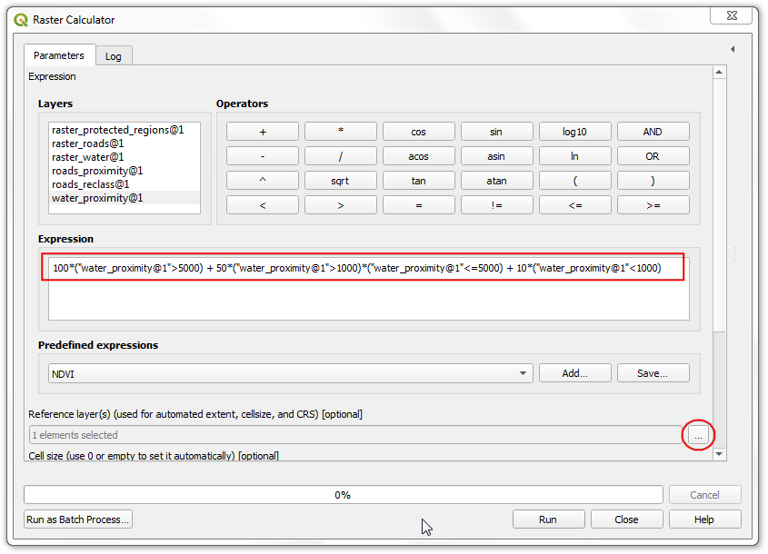
  Select water_proximity layer using … button as an Input Layer. Enter the following expression hat applies the above criteria on the input. Keep all the other options as default and save the output layer with the name water_reclass.tif and click Run.

  100*("water_proximity@1">2000)
  + 50*("water_proximity@1">1000)*("water_proximity@1"<=2000)
  + 10*("water_proximity@1"<1000)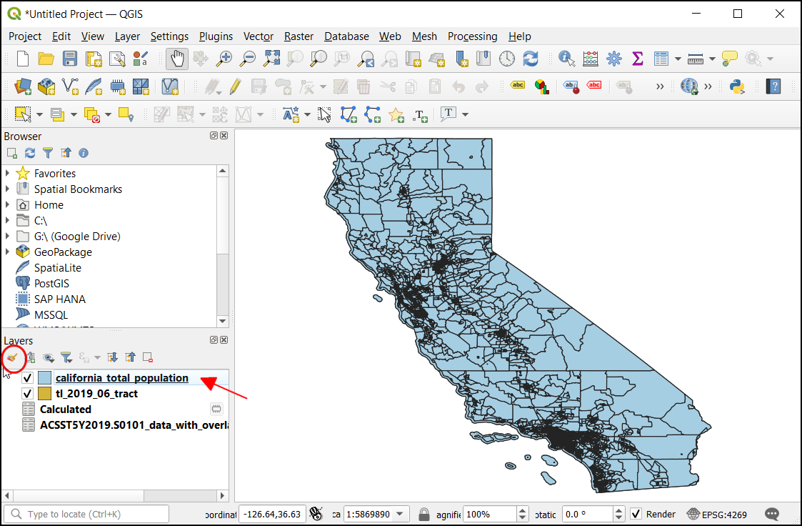
  

  

22. Now we are ready to do the final overlay analysis. Recall that our criteria for determining suitability is as follows - close to roads, away from water and not in a protected region. Open Raster analysis ‣ Raster calculator. Select roads_reclass, water_reclass, raster_protected_regions_filled layers using … button as Input Layers. Use ε button to enter the following expression that applies these criteria. Keep other parameters as default. Name the output overlay.tif and click Run.

(("roads_reclass@1" + "water_reclass@1")/2)
*("raster_protected_regions@1"  !=  1 )

Bemerkung

In this example, we are giving equal weight to both road and water proximity. In real-life scenario, you may have multiple criteria with different importance. You can simulate that by multiplying the rasters with appropriate weights in the above expression. For example, if proximity to roads is twice as importance as proximity away from water, instead of (("roads_reclass@1" + "water_reclass@1")/2), you can use the expression ((2*"roads_reclass@1" + "water_reclass@1")/3).

23. Once the processing finishes, the resulting raster overlay will be added to the Layers panel. The pixel values in this raster range from 0 to 100 - where 0 is the least suitable and 100 is the most suitable area for development. Let’s clip the results to the boundary layer. Open Raster extraction ‣ Clip raster by mask layer algorithm.

24. In the Raster Extraction - Clip Raster by Mask Layer dialog, select overlay as the Input layer and boundary as the Mask layer.

25. Scroll down to find the Advanced Parameters and select the profile High Compression to apply the compression. Save the Clipped (mask) layer as overlay_clipped.tif and click Run.

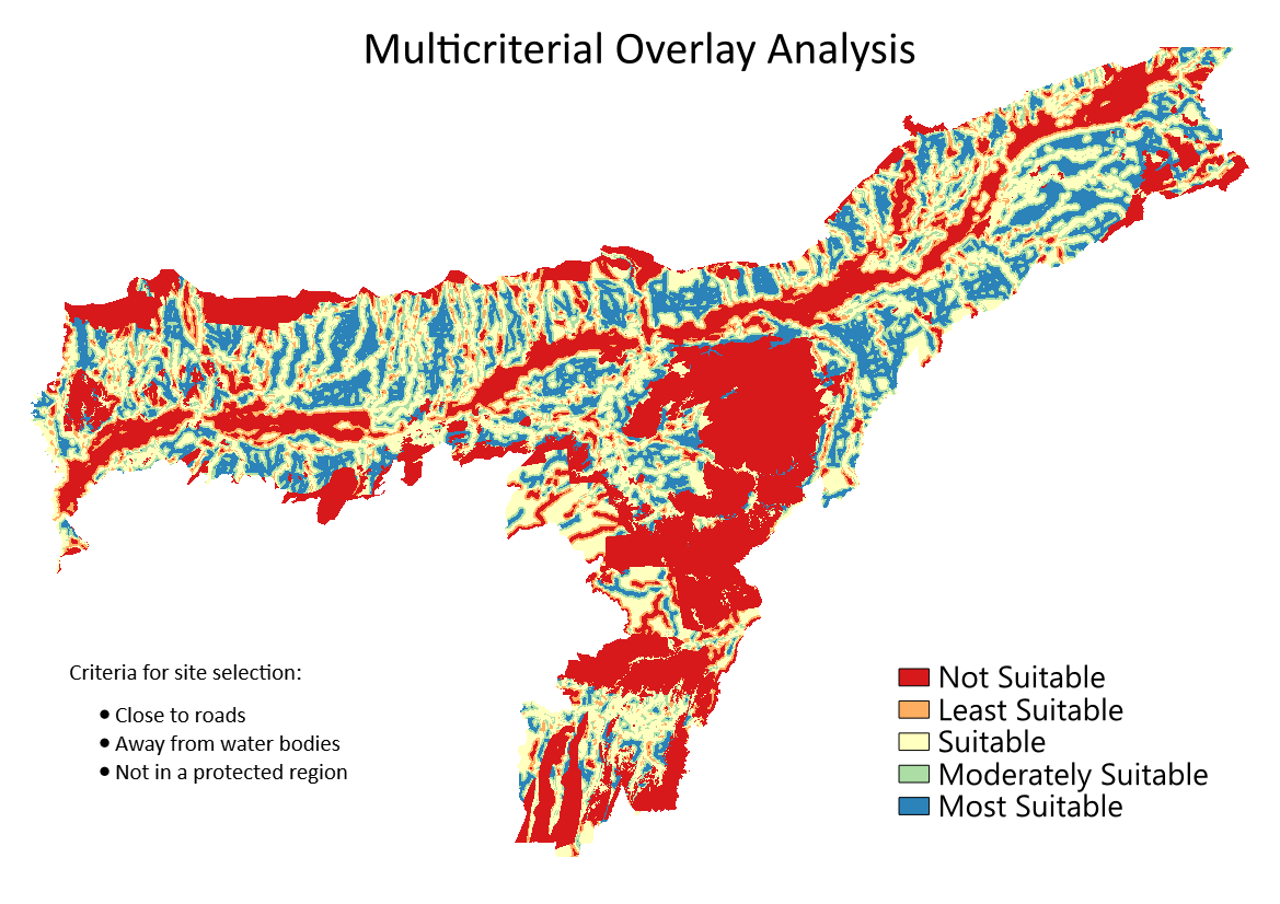
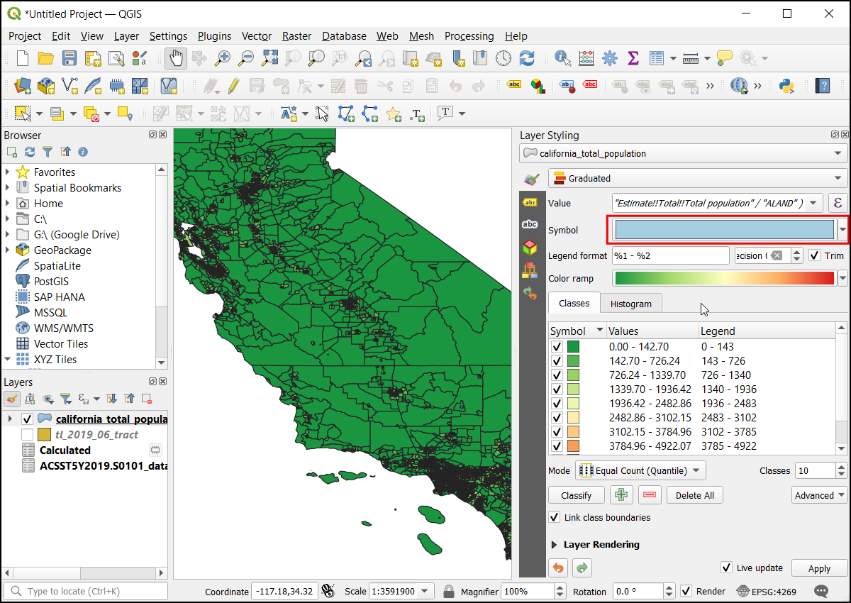
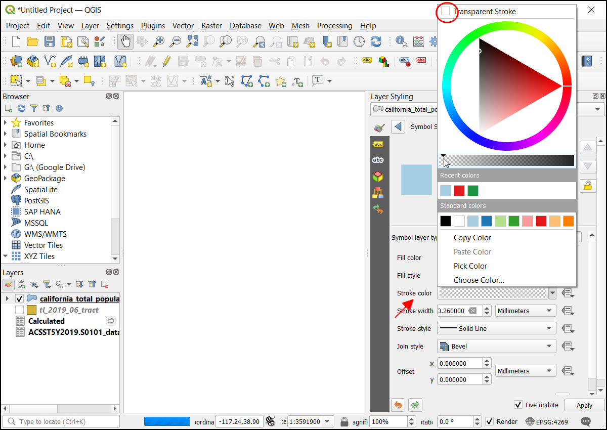
26. Once the processing finishes, the final output layer overlay_clipped will be added to the Layers panel. Click the Open the Layer Styling panel button in the Layers panel and select the Singleband pseudocolor renderer.

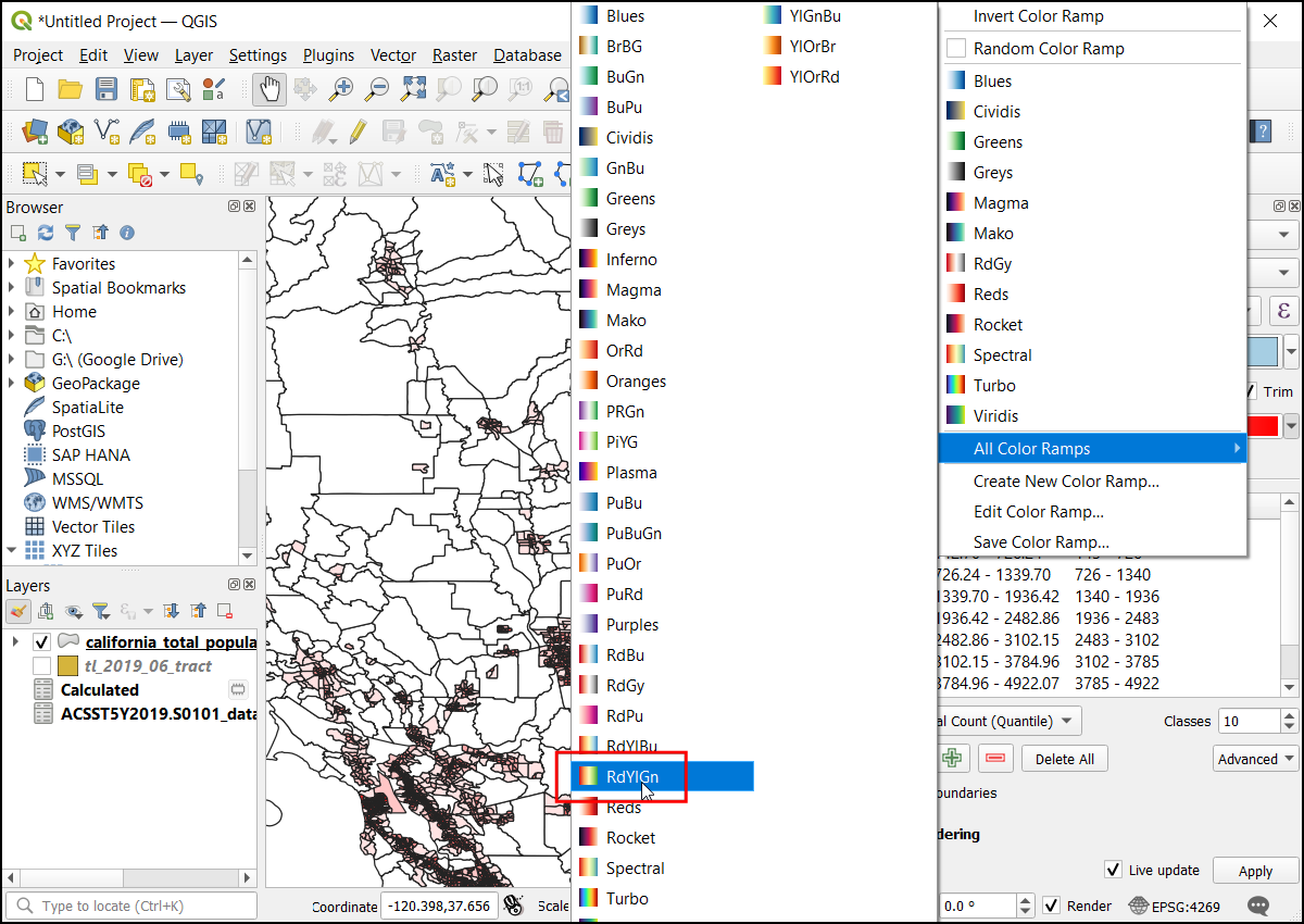
27. Set the Interpolation to Discrete and choose the Spectral color ramp.

28. Click on the default label values next to each color and enter appropriate labels.

29. The labels will also appear as the legend under the overlay_clipped layer. This is our final map showing the site suitability according to the chosen criteria.

---

If you want to give feedback or share your experience with this tutorial, please comment below. (requires GitHub account)