تحلیل همپوشانی چندمعیار­ه (QGIS3)

تحلیل همپوشانی وزنی چندمعیار­هMulti-criteria weighted-overlay analysis فرآیند تخصیص یک زمین بر اساس خصوصیات متنوعی است که باید ارزیابی شوند. اگرچه این یک عملیات معمولی GIS است، اما بهتر است با استفاده از یک روش مبتنی بر رستر انجام شود.

توجه

همپوشانی رستر و بردار

You can do the overlay analysis on vector layers using geoprocessing tools such as buffer, dissolve, difference and intersection. This method is ideal if you wanted to find a binary suitable/non-suitable answer and you are working with a handful of layers. You can review our video tutorial on Locating A New Bicycle Parking Station using Multicriteria Overlay Analysis for a step-by-step guide on this approach.

کار با رستر علاوه بر یافتن بهترین سایت مناسب به شما کمک می‌کند تناسب را رتبه‌بندی نمایید؛ همچنین به شما این امکان می‌دهد تعداد زیادی از لایه ورودی را به‌راحتی ترکیب کرده و وزن‌های مختلفی را به هر یک از معیارها اختصاص دهید. به‌طورکلی، این روش مناسب برای تناسب اراضی است.

این آموزش برای انجام تجزیه‌وتحلیل تناسب اراضی است که گردش کار عملیات آن شامل تبدیل داده‌های برداری به رستر، طبقه‌بندی و ارزش‌گذاری آن‌ها و انجام عملیات ریاضی هستند.

نمای کلی تمرین

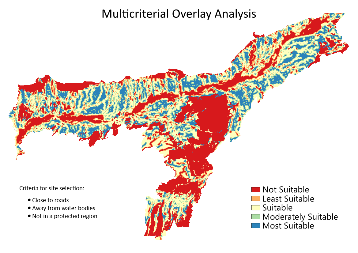
در این آموزش، با اجرای تناسب اراضی، «منطقه مناسب جهت توسعه» مکان‌یابی می‌شود، بدین منظور در ابتدا، یک سری قواعد (معیار) تعریف می‌شود: یعنی منطقه مناسب برای توسعه دارای شرایط ذیل باشد

• ·  نزدیک به جاده باشد و

• · دور از منابع آبی باشد و

• ·در منطقه حفاظت‌شده قرار نگیرد.

اخذ داده

ما از لایه‌های داده‌برداری OpenStreetMap (OSM) <http://www.openstreetmap.org/> استفاده خواهیم کرد؛ OSM یک پایگاه داده جهانی از داده‌های نقشه پایه است که به‌طور آزاد در دسترس است. Geofabrik فایلهای روزانه مجموعه داده OpenStreetMap را به‌روز می‌کند.

We will be using the OSM data layers for the state of Assam in India. Geofabrik India shapefiles were downloaded, reprojected to a UTM projection, clipped to the state boundary and packaged in a single GeoPackage file. You can download a copy of the geopackage from the link below:

assam.gpkg

منابع داده : [GEOFABRIK]

مراحل

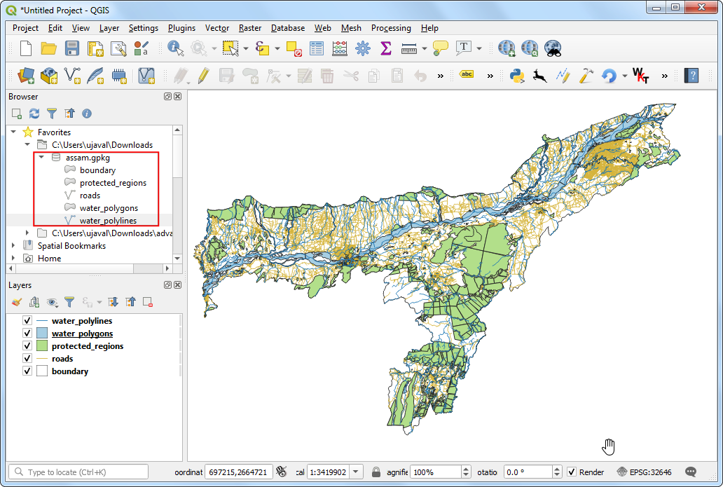
1. در محیط نرم‌افزار QGIS، در پانل Browser آن به فایل پایگاه داده  assam.gpkgدانلود شده بروید؛ آن را بازکنید و هر پنج لایه داده جداگانه را به فریم نقشه بکشید. شما لایه‌برداری مرز منطقه boundary، راه‌ها roads`، مناطق حفاظت‌شده protected_regions، پلی‌گون منابع آب water_polygons و رودخانه `water_polylines``در پانل Layers خواهید دید

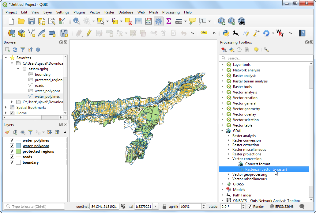
2. First step in the overlay analysis, is to convert each data layer to raster. An important consideration is that all rasters must be of the same extent. We will use the boundary layer as the extent for all the rasters. Go to Processing ‣ Toolbox. Search for and locate the GDAL ‣ Vector conversion ‣ Rasterize (vector to raster) algorithm. Double-click to launch it.

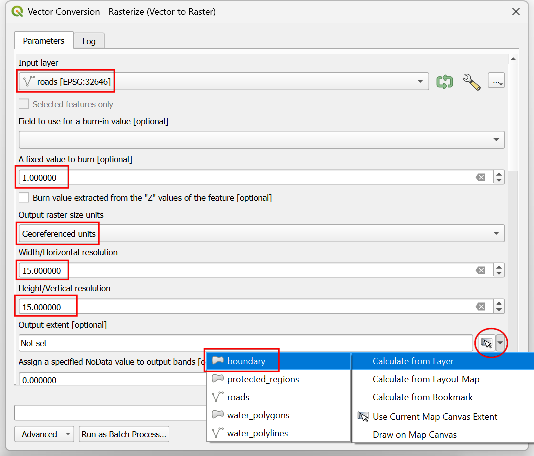
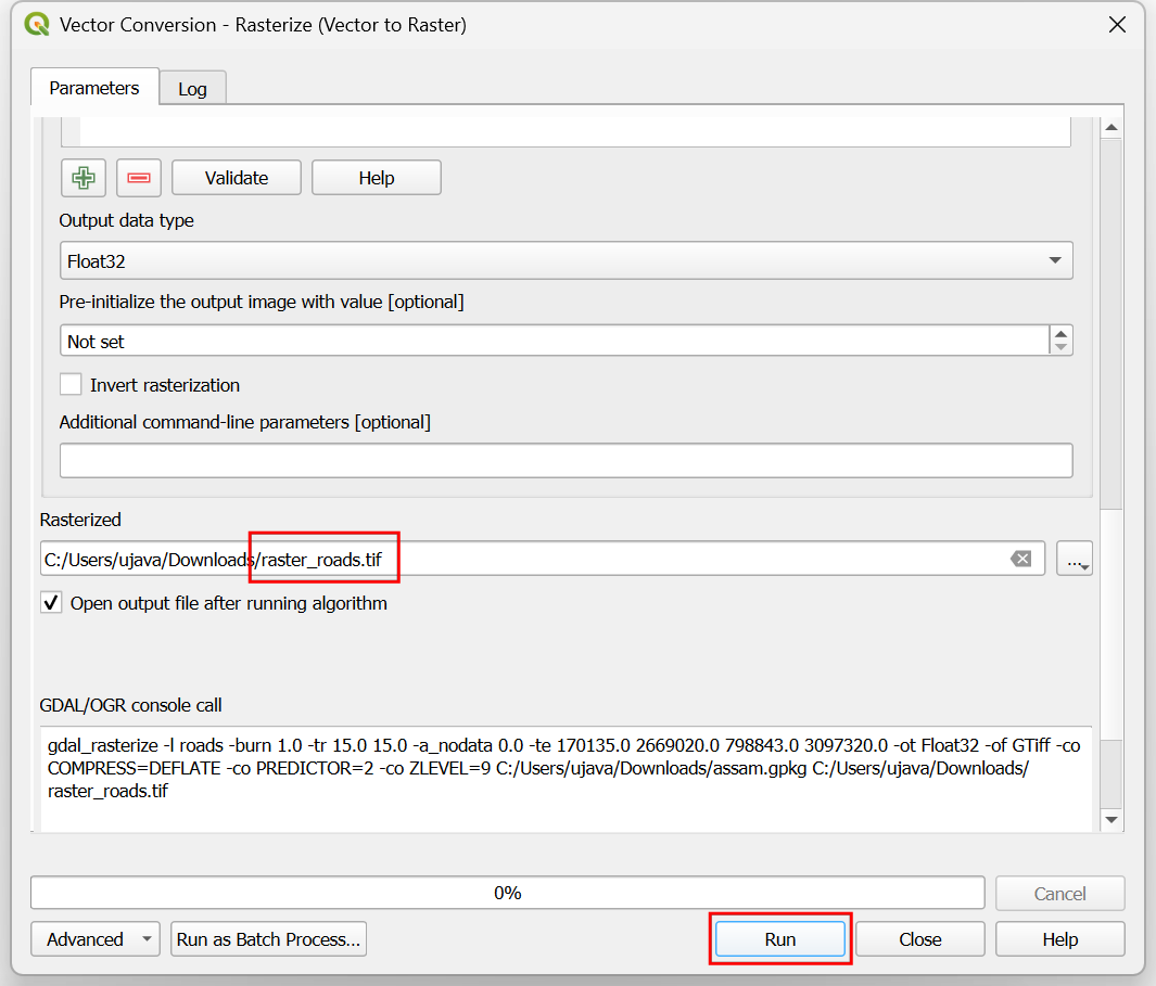
3. In the Vector Conversion - Rasterize (vector to raster) dialog, select roads as the Input layer. We want to create an output raster where pixel values are 1 where there is a road and 0 where there are no roads. Enter 1 as the A fixed value to burn. The input layers are in a projected CRS with meters are the unit. Select Geoferenced units as the Output raster size units. We will set the resolution of the output raster to be 15 meters. Select 15 as both Width/Horizontal resolution and Height/Vertical resolution. Next, click the arrow next to Output extent and select Calculate from Layer ‣ boundary.

4. Scroll down to find the Advanced Parameters and select the profile High Compression to apply the compression. This will generate the compressed raster file of smaller size after running the tool. Applying lossless compression is highly recommended while working with raster data.

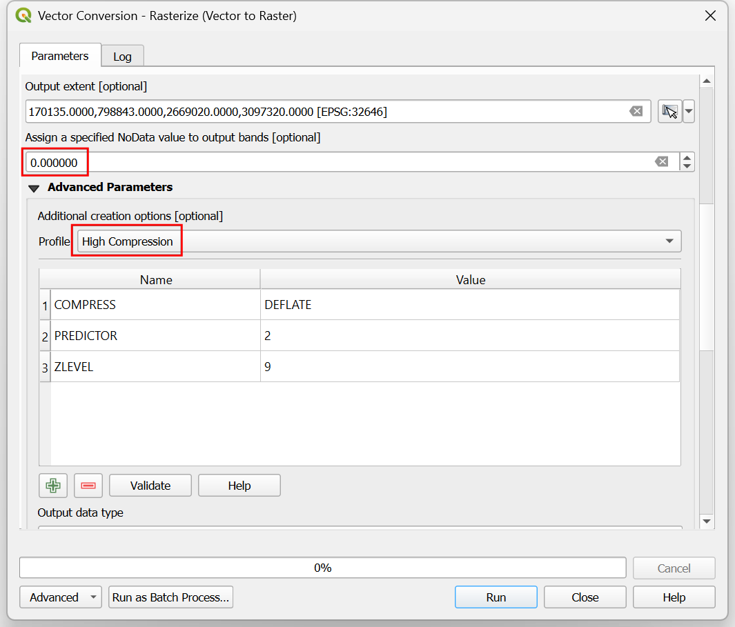
5. Set the Rasterized output raster as raster_roads.tif and click Run.

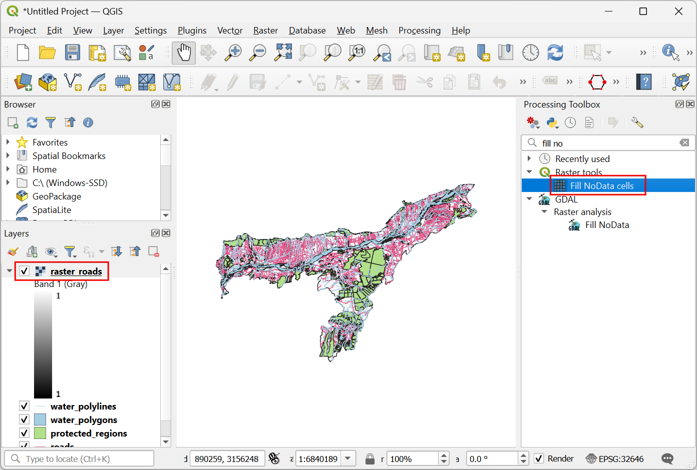
6. Once the processing finishes, you will see a new layer raster_roads loaded in the Layers panel. The raster has pixel values 1 for pixels which intersected with the roads. All other pixels are set as NoData values. These nodata values are problematic because when raster calculator (which we will use later) encounters a pixel with nodata value in any layer, it sets the output value of that pixel to nodata as well, resulting is unexpected output. We will fill these nodata values with the value 0. Search for and locate the Raster Tools ‣ Fill NoData cells algorithm. Double-click to launch it.

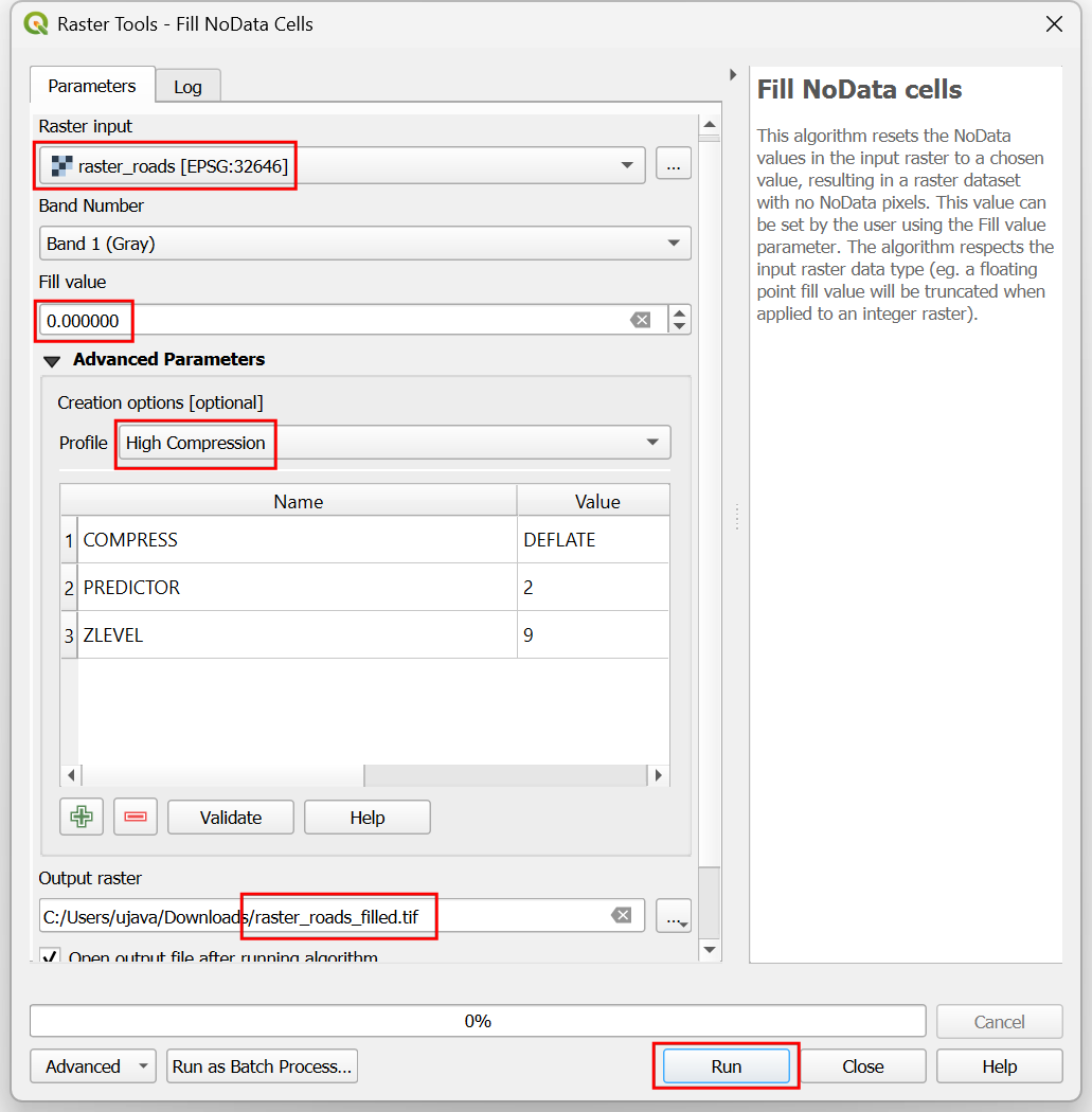
7. Select raster_roads as the Raster input and choose 0 as the Fill value. Scroll down to find the Advanced Parameters and select the profile High Compression to apply the compression. Set the Output raster as raster_roads_filled.tif and click Run.

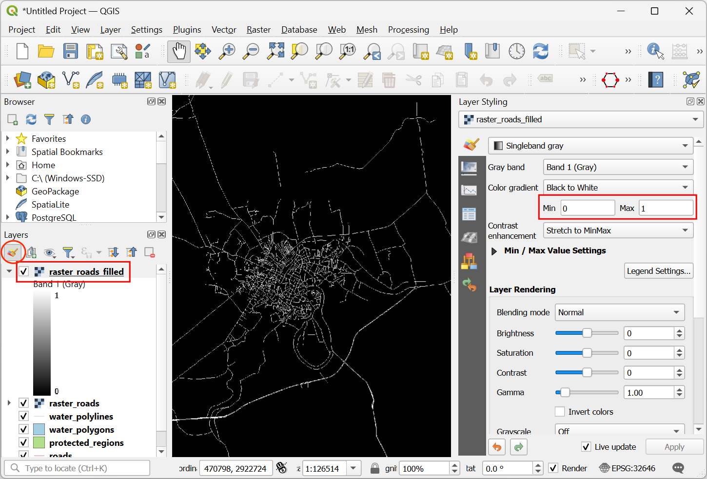
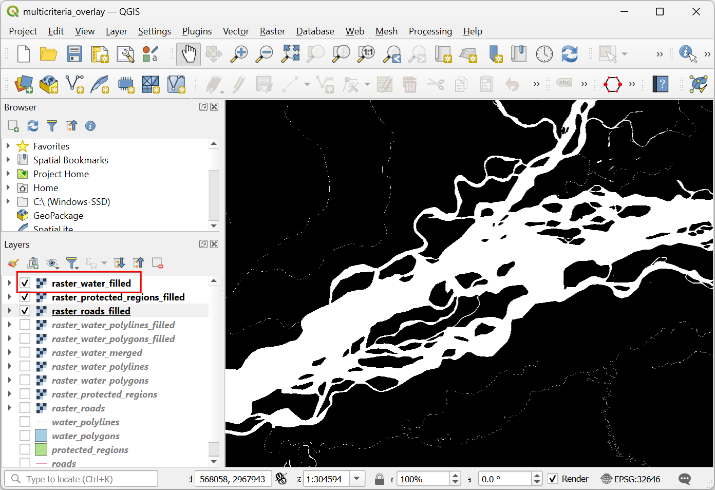
8. Once the processing finishes, you will see the new layer raster_roads_filled loaded in the Layers panel. This raster has values 1 for roads and 0 for no roads. If the layer is not visualized correctly, you can click the Open the Layer Styling Panel and set the Min to 0 and Max to 1.

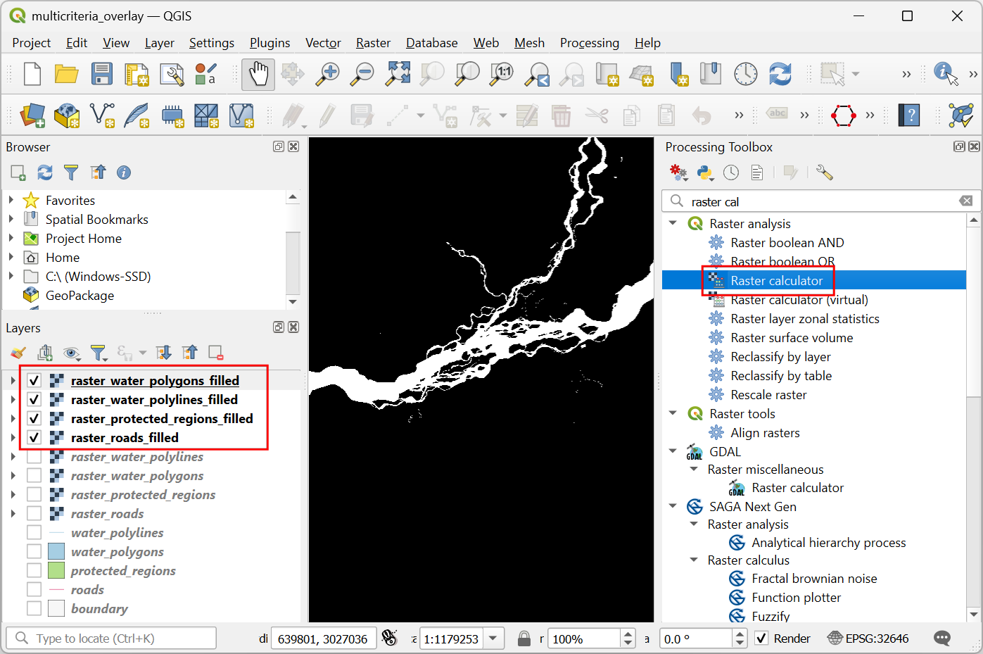
9. Repeat steps 3-8 for the other 3 vector layers protected_regions, water_polylines and water_polygons layers. You need to rasterize and fill the nodata cells for these layers. If you want to run these steps manually, you can configure the processing algorithm dialog, run the algorithm and once the algorithm finishes, switch to the Parameters tab and just change the input and output layer names. You can also run each algorithm on all 4 layers in a single step using Batch Processing. See the Batch Processing using Processing Framework (QGIS3) tutorial to learn more. Once you are done, you should have 4 raster layers and generate the corresponding raster layers raster_roads_filled, raster_protected_regions_filled, raster_water_polylines_filled and raster_water_polygons_filled. You will notice that we have 2 water related layers - both representing water. We can merge them to have a single layer representing water areas in the region. Search for and locate Raster analysis ‣ Raster calculator algorithm in the Processing Toolbox. Double-click to launch it.

10. Select raster_water_polygons and raster_water_polylines layers using ... button as Input Layers. Enter the following expression using ε button. Keep all the other options as default and save the output layer with the name raster_water_merged.tif and click Run.

"raster_water_polygons_filled@1" + "raster_water_polylines_filled@1"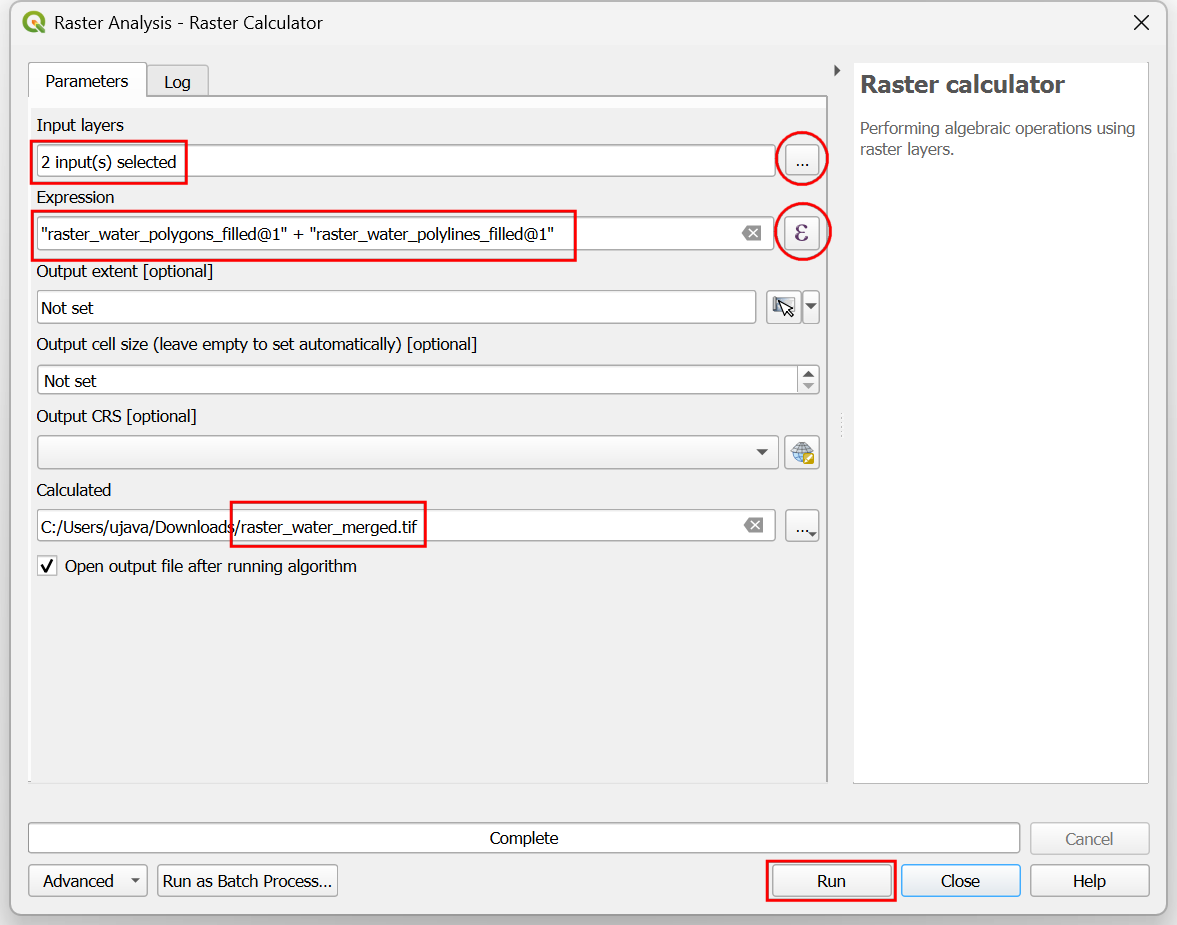

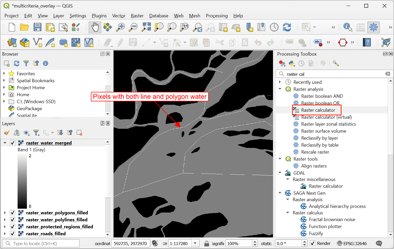
11. رستر ادغام‌شده باید دارای پیکسل‌هایی با مقادیر 1 برای تمام مناطق آب خواهد بود. ملاحظه خواهید کرد که مناطقی وجود دارند که دولایه یعنی، هم لایه چندضلعی آب و لایه خطی آب وجود دارند. لذا این مناطق پیکسل‌هایی با مقادیر 2 خواهند داشت - که درست نیست. ما می‌توانیم با یک دستور ساده آن را برطرف کنیم؛ دستور Raster analysis ‣ Raster calculator دوباره باز کنید.

12. Select raster_water_merged layer using ... button as an Input Layer. Enter the following expression using ε button. Keep all the other options as default and save the output layer with the name raster_water_filled.tif and click Run.

"raster_water_merged@1" > 0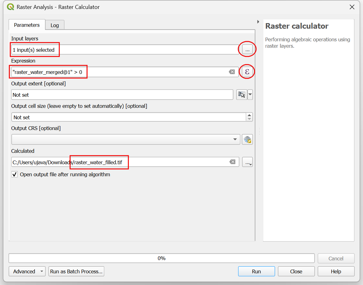

13. The resulting layer raster_water_filled now has pixels with only 0 and 1 values.

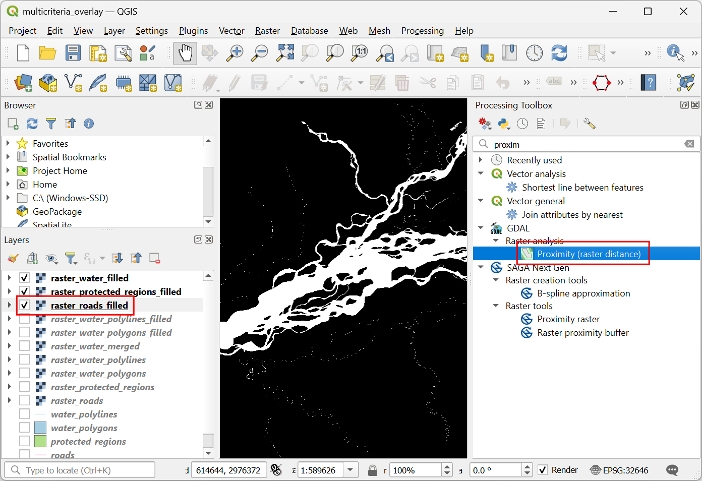
14. اکنون‌که لایه‌هایی رستری جاده و منابع آب داریم، می‌توانیم لایه رستری فاصله (مجاورت) ایجاد کنیم. این‌ها همچنین به‌عنوان فاصله اقلیدسی شناخته می‌شوند - جایی که هر پیکسل در رستر خروجی نشان‌دهنده فاصله تا نزدیک‌ترین پیکسل در رستر ورودی است. سپس، می‌توان از این رستر به‌دست‌آمده برای تعیین مناطق مناسب که در فاصله مشخصی از ورودی قرار دارند، استفاده کرد. الگوریتم GDAL ‣ Raster analysis ‣ Proximity (raster distance) را جستجو و پیدا کنید. برای اجرای آن دو بار کلیک کنید.

15. In the Raster Analysis - Proximity (Raster Distance) dialog, select raster_roads_filled as the Input layer. Choose Georeferenced coordinates as the Distance units. As the input layers are in a projected CRS with meters as the units, enter 5000 (5 kilometers) as the Maximum distance to be generated. For all pixels that are more than the maximum distance away - we will set their values to be 5000 as well. So set the Nodata value to use for the destination proximity raster value to 5000.

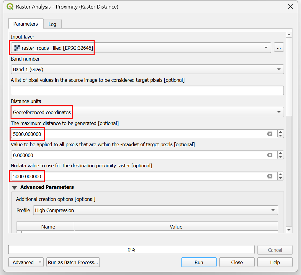
16. You can expand the Advanced Parameters and select the profile High Compression to apply the compression. Name the output file as roads_proximity.tif and click Run.

توجه

It may take upto 15 minutes for this process to run. It is a computationally intensive algorithm that needs to compute distance for each pixel of the input raster.

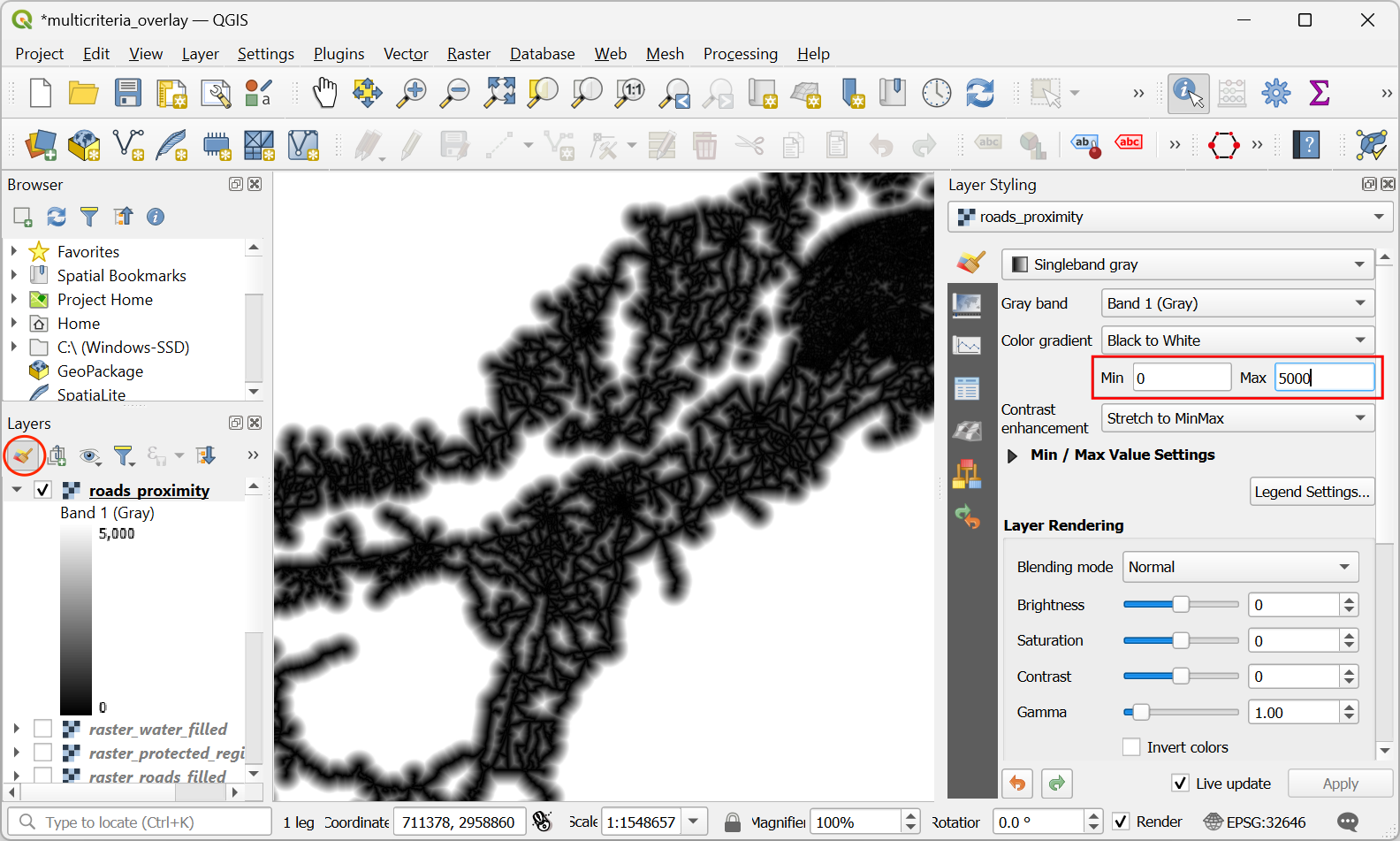
17. Once the processing is over, a new layer roads_proximity will be added to the Layers panel. To visualize it better, let's change the default styling. Click the Open the Layer Styling panel button in the Layers panel. Change the Max value to 5000 under Color gradient.

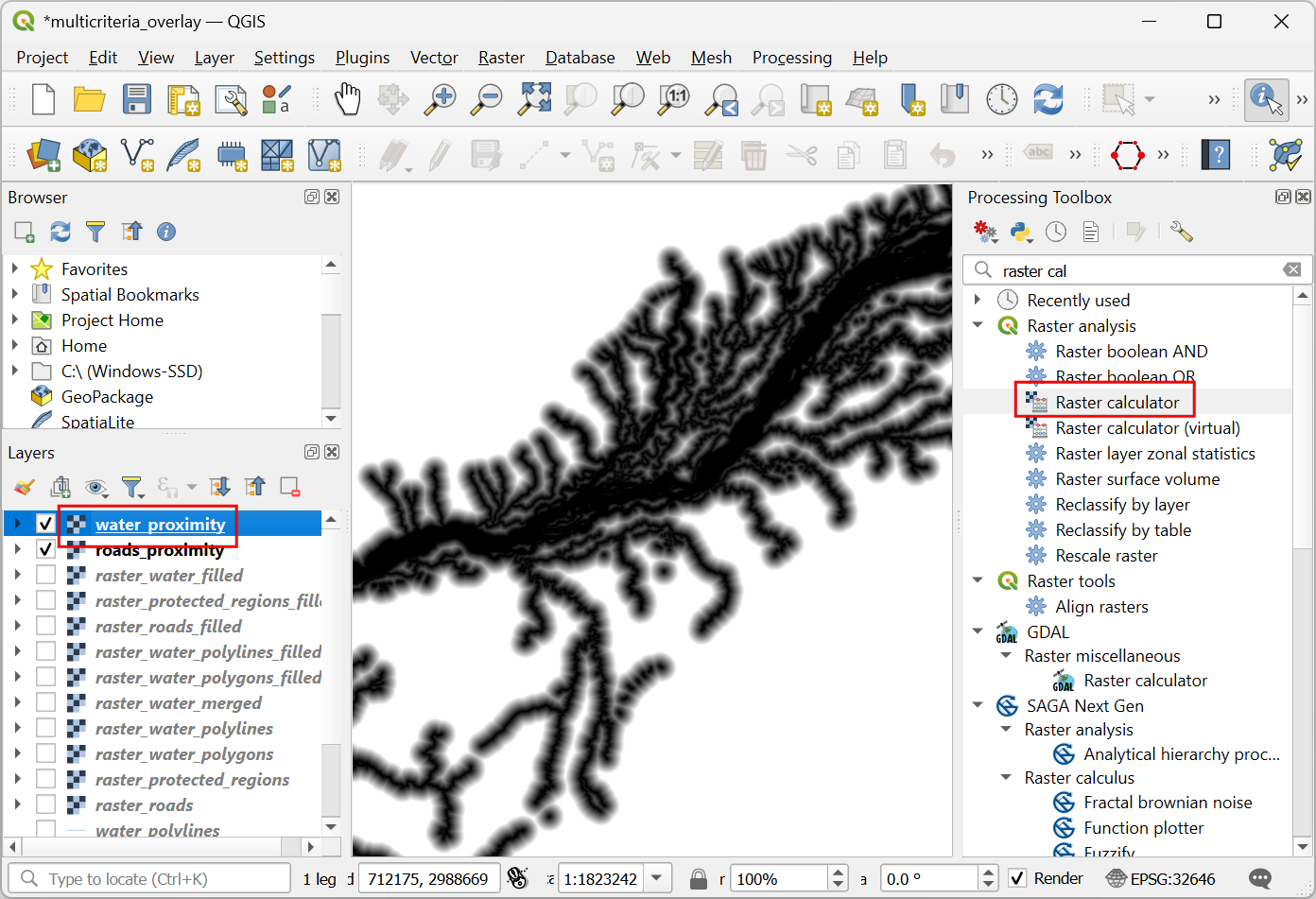
18. Repeat the Proximity (Raster Distance) algorithm for the raster_water_filled layer with same parameters and name the output water_proximity.tif. If you click around the resulting raster, you will see that it is a continuum of values from 0 to 5000. To use this raster in overlay analysis ,we must first re-classify it to create discrete values. Open Raster analysis ‣ Raster calculator algorithm again.

19. We want to give higher score to pixels that are near to roads. So let's use the following scheme.

• 0-1000m –> 100

• 1000-2000m –> 50

• >2000m –> 10

  Select roads_proximity layer using ... button as an Input Layer. Enter the following expression that applies the above criteria on the input. Keep all the other options as default and save the output layer with the name roads_reclass.tif and click Run.

  100*("roads_proximity@1"<=1000)
      + 50*("roads_proximity@1">1000)*("roads_proximity@1"<=2000)
      + 10*("roads_proximity@1">2000)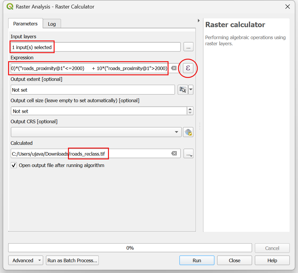
  

  

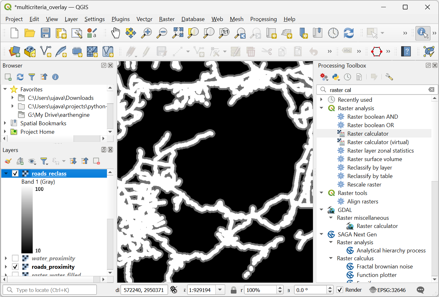
20. Once the re-classification process finishes, a new layer roads_reclass will be added to the Layers panel. This layer has only 3 different values, 10, 50 and 100 indicating relative suitability of the pixels with regards to distance from roads. Open Raster analysis ‣ Raster calculator algorithm again.

21. Repeat the re-classification process for the water_proximity layer. Here the scheme will be reverse, where pixels that are further away from water shall have higher score.

• · 0-1000 -> 10

• 1000 -2000m —> 50

• >2000m –> 100

  Select water_proximity layer using ... button as an Input Layer. Enter the following expression hat applies the above criteria on the input. Keep all the other options as default and save the output layer with the name water_reclass.tif and click Run.

  100*("water_proximity@1">2000)
  + 50*("water_proximity@1">1000)*("water_proximity@1"<=2000)
  + 10*("water_proximity@1"<1000)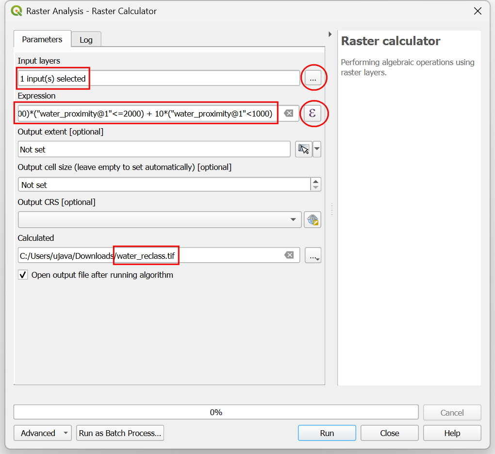
  

  

22. Now we are ready to do the final overlay analysis. Recall that our criteria for determining suitability is as follows - close to roads, away from water and not in a protected region. Open Raster analysis ‣ Raster calculator. Select roads_reclass, water_reclass, raster_protected_regions_filled layers using ... button as Input Layers. Use ε button to enter the following expression that applies these criteria. Keep other parameters as default. Name the output overlay.tif and click Run.

(("roads_reclass@1" + "water_reclass@1")/2)
*("raster_protected_regions@1"  !=  1 )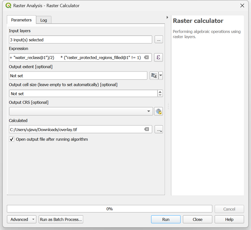

توجه

In this example, we are giving equal weight to both road and water proximity. In real-life scenario, you may have multiple criteria with different importance. You can simulate that by multiplying the rasters with appropriate weights in the above expression. For example, if proximity to roads is twice as importance as proximity away from water, instead of (("roads_reclass@1" + "water_reclass@1")/2), you can use the expression ((2*"roads_reclass@1" + "water_reclass@1")/3).

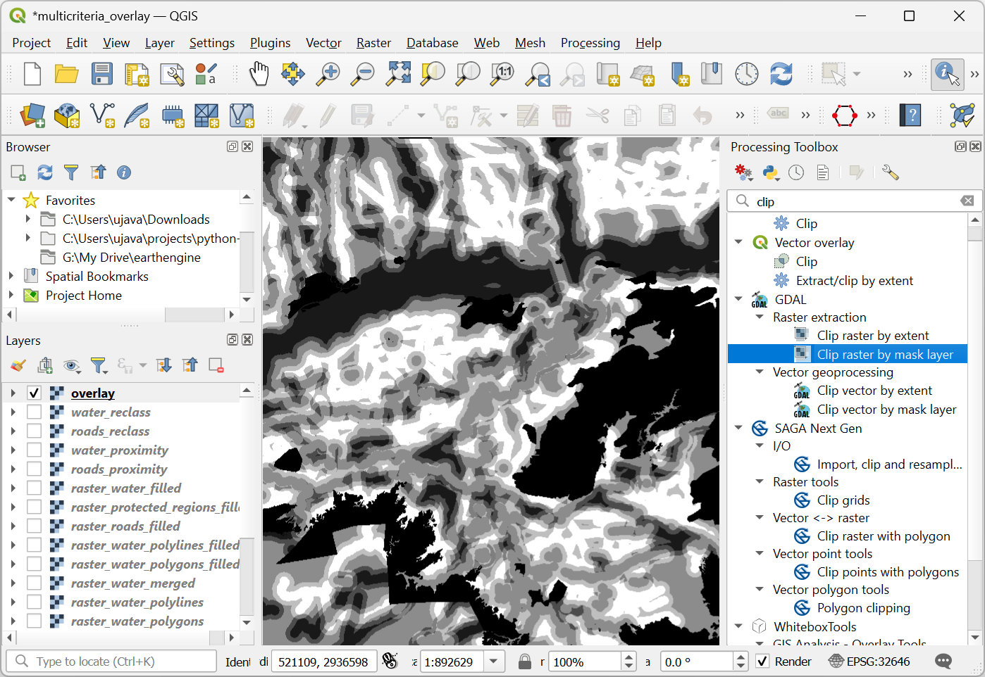
23. Once the processing finishes, the resulting raster overlay will be added to the Layers panel. The pixel values in this raster range from 0 to 100 - where 0 is the least suitable and 100 is the most suitable area for development. Let's clip the results to the boundary layer. Open Raster extraction ‣ Clip raster by mask layer algorithm.

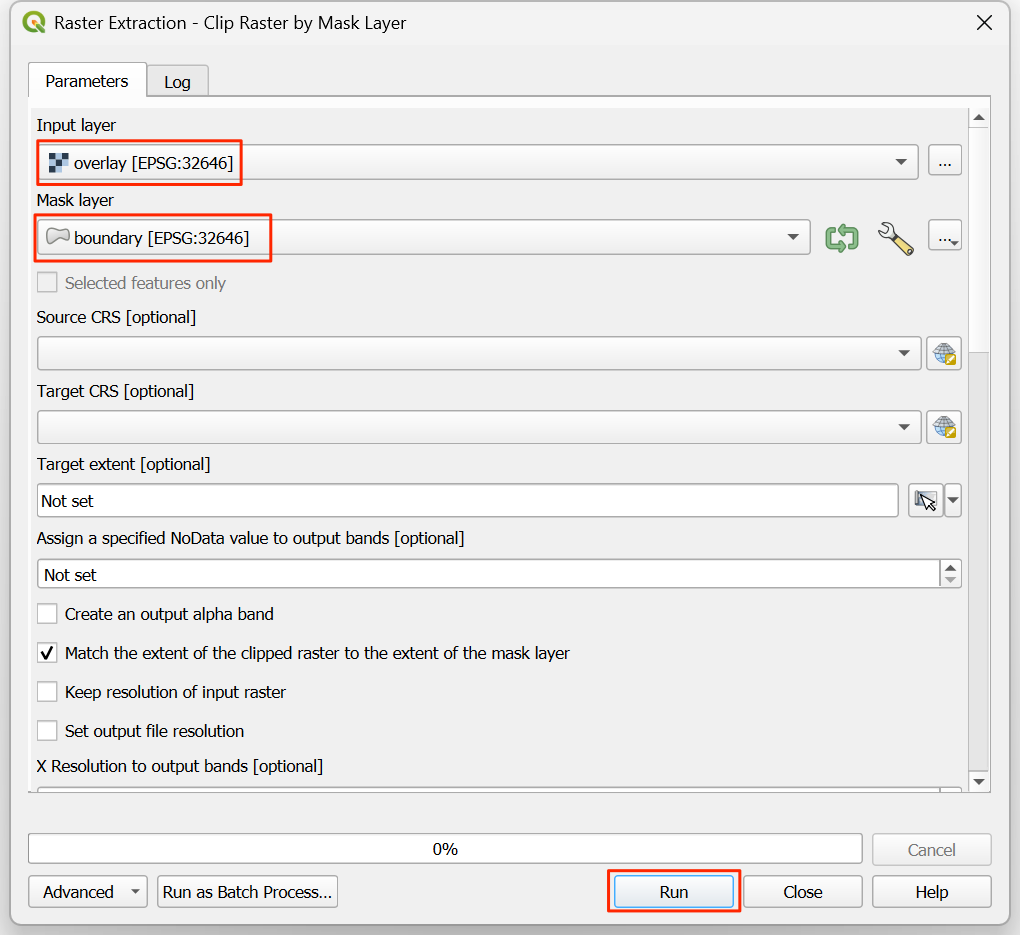
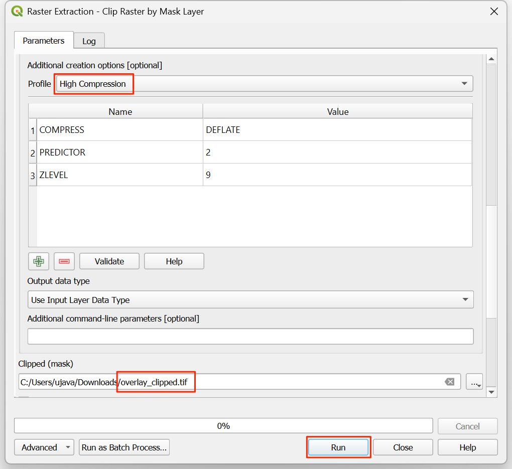
24. In the Raster Extraction - Clip Raster by Mask Layer dialog, select overlay as the Input layer and boundary as the Mask layer.

25. Scroll down to find the Advanced Parameters and select the profile High Compression to apply the compression. Save the Clipped (mask) layer as overlay_clipped.tif and click Run.

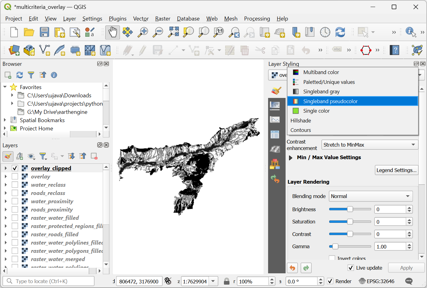
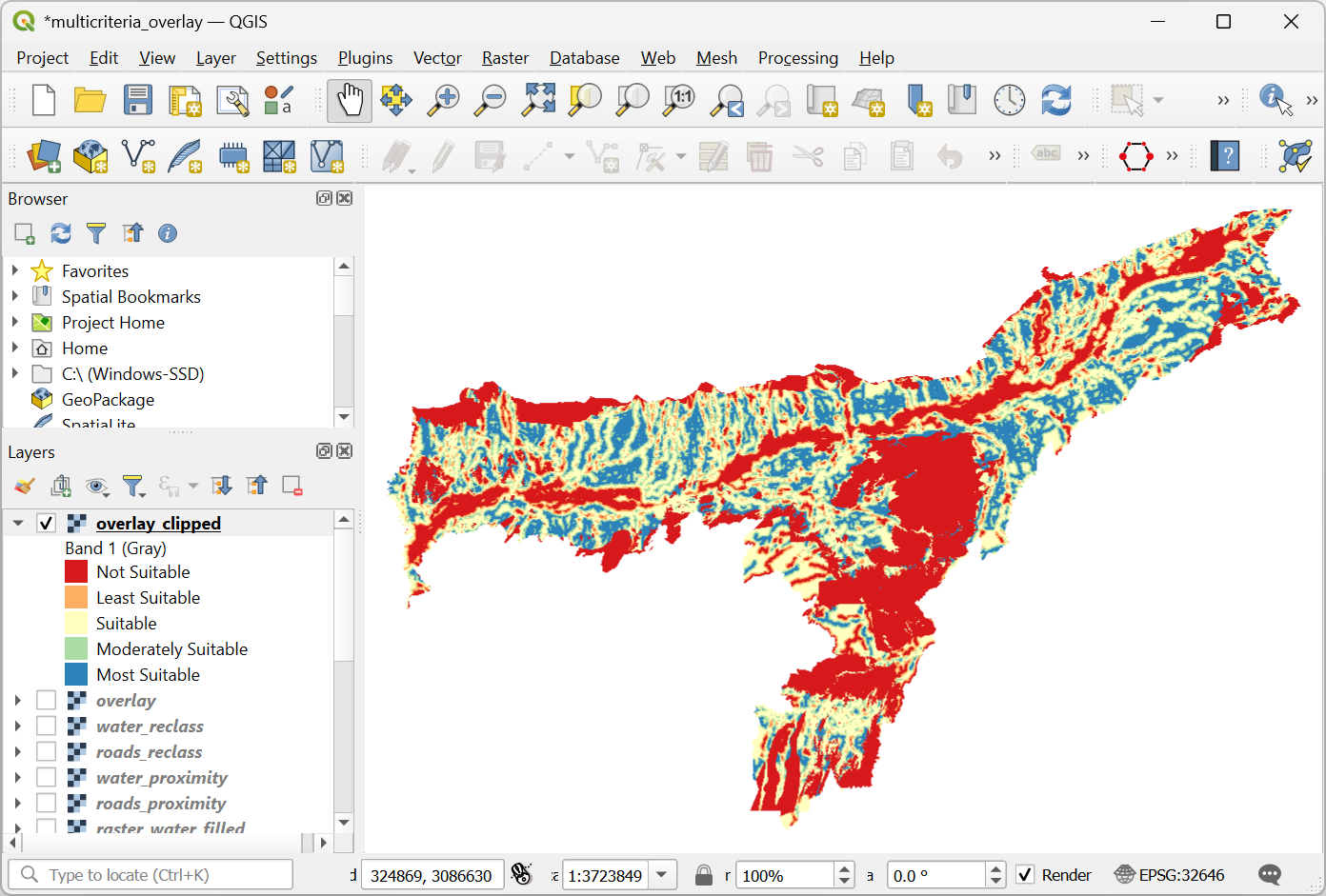
26. Once the processing finishes, the final output layer overlay_clipped will be added to the Layers panel. Click the Open the Layer Styling panel button in the Layers panel and select the Singleband pseudocolor renderer.

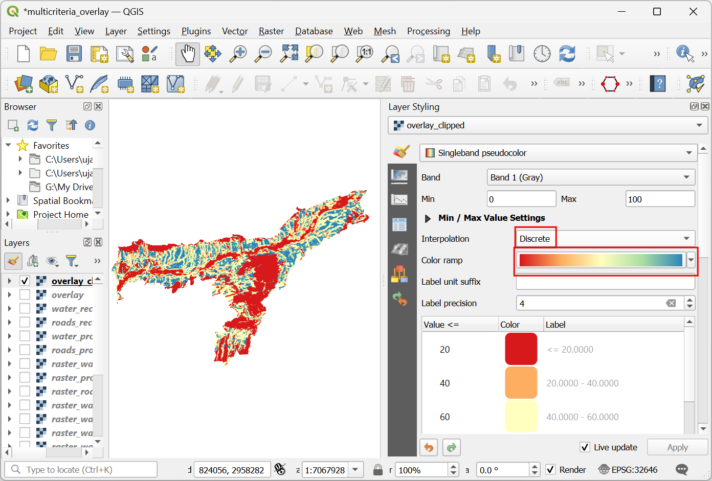
27. Set the Interpolation to Discrete and choose the Spectral color ramp.

28. Click on the default label values next to each color and enter appropriate labels.

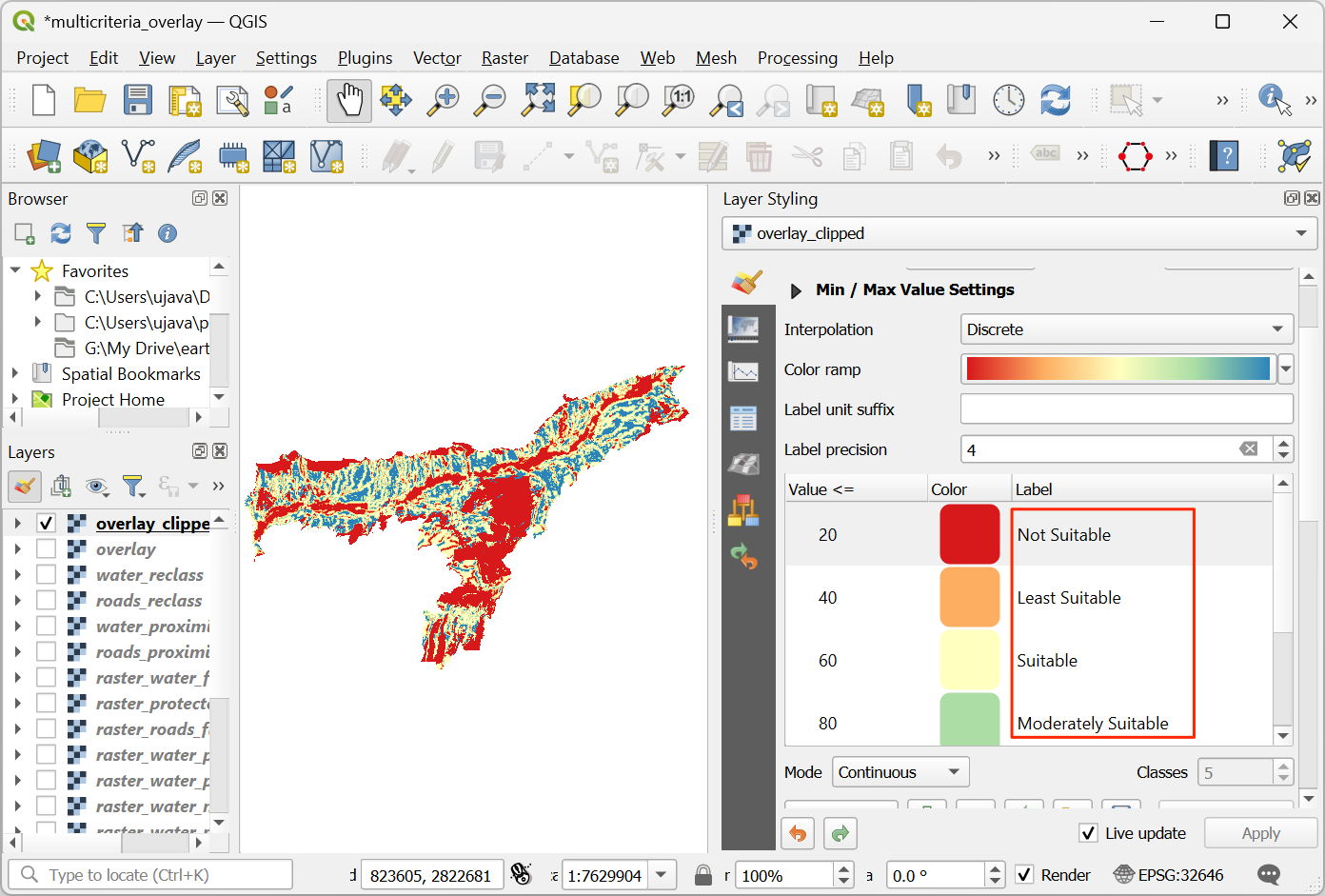
29. The labels will also appear as the legend under the overlay_clipped layer. This is our final map showing the site suitability according to the chosen criteria.

---

If you want to give feedback or share your experience with this tutorial, please comment below. (requires GitHub account)