Locating Nearest Facility with Origin-Destination Matrix (QGIS3)¶

In the previous tutorial, Basic Network Visualization and Routing (QGIS3), we learned how to build a network and calculate the shortest path between 2 points. We can apply that technique to many different types of network-based analysis. One such application is to compute Origin-Destination Matrix or OD Matrix. Given a set of origin points and another set of destination points, we can calculate the shortest path between each origin-destination pairs and find out the travel distance/time between them. Such analysis is useful to locate the closest facility to any given point. For example, a logistics company may use this analysis to find the closest warehouse to their customers to optimize delivery routes. Here we use the Distance Matrix algorithm from QGIS Network Analysis Toolbox (QNEAT3) plugin to find the nearest health facility to each address in the city.

備註

This tutorial shows how to use your own network data to compute an origin-destination matrix. If you do not have your own network data, you can use ORS Tools Plugin and algorithm ORS Tools ‣ Matrix ‣ Matrix from Layers to do a similar analysis using OpenStreetMap data. See Service Area Analysis using Openrouteservice (QGIS3) to learn how to use ORS Tools plugin.

Overview of the task¶

We will take 2 layers for Washington DC - one with points representing addresses and another with points representing mental health facilities - and find out the facility with the least travel distance from each address.

Other skills you will learn¶

Extract a random sample from a point layer.
Use Virtual Layers to run SQL query on a QGIS layer.

Get the data¶

District of Columbia government freely shares hundreds of datasets on the Open Data Catalog.

Download the following data layers as shapefiles.

For convenience, you may directly download a copy of the datasets from the links below:

Roadway_Block-shp.zip

Address_Points.zip

Community Based Service Provider.zip

Data Source: [DCOPENDATA]

Setup¶

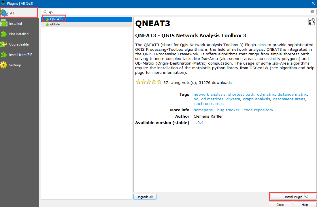
Visit Plugins ‣ Manage and Install plugins. Select :guilabel:` All` Search for QNEAT3 plugin and install it. Click Close.

Procedure¶

Locate the Community_Based_Service_Providers.zip file, expand it and add Community_Based_Service_Providers.shp to the canvas. We will select only those centres providing facilities to adults. Right-click on the Community_Based_Service_Providers.shp layer and select Filter.

It will open a Query Builder dialog box. Enter the following query in the :guilabel:` Filter Expression` Click Run.

"PROVIDER_T"  IN ('Adult','Adult & Child')

Next, locate the Roadway_Block.zip file, expand it and add the Roadway_Block.shp. Similarly, locate the Address_Points.zip file, expand it and add the Address_Points.shp. You will see a lot of points around the city. Each point represents a valid address. We will select 1000 points randomly. This technique is called random sampling. Go to Processing ‣ Toolbox.

Search for and locate the Vector Selection ‣ Random extract algorithm.

Select Address_Points as the Input layer, Number of feature as the Method and, enter 1000 in the Number/percentage of features. In the Extracted (random) choose the ... and click Save to a file. Now choose the directory and enter the name as address_point_subset.shp and click Run.

備註

As the algorithm will extract 1000 random points from the given data set, to replicate the exact points used in this exercise you can download the subset file which we got during the execution of the algorithm here address_point_subset.zip . After downloading load address_point_subset.shp layer into QGIS.

A new layer address_point_subset will be added to the Layers panel, you can turn off the visibility of Address_Points address points layer. Let’s rename this layer as origin_points. Right-click on the address_point_subset layer and select Rename layer.

Similarly, rename the Adult_Mental_Health_Providers layers representing the health facilities as destination_points. Naming the layers this way makes it easy to identify them in subsequent processing. Further we will open processing toolbox to create the distance matrix using origin and destination layers.

Locate the QNEAT3 ‣ Distance matrices ‣ OD Matrix from Layers as Line (m:n) algorithm. If you do not see this algorithm in the toolbox, make sure you have installed the QNEAT3 plugin.

This algorithm helps find the distances along with the network between selected origin and destination layers. Select Roadway_Block as the Network layer. Select origin_points as the From-Points layer and OBJECTID_1 as the Unique Point ID field. Similarly, set destination_points as the To-Points Layer and OBJECTID as the Unique Point ID field. Set the Optimization Criterion as Shortest Path (distance optimization).

As many streets in the network are one-way, we need to set the Advanced parameters to specify the direction. See Basic Network Visualization and Routing (QGIS3) for more details on how these attributes are structured. We also have an option to select geometry style of the generated matrix. We are having a road network with direction information so we can generate matrix by folling the route. Choose Matrix geometry follows routes.Choose SUMMARYDIR as the Direction field. Enter OB as the Value for the forward direction, IB as the Value for backward direction, and BD as the Value for the both direction. Set the Topology tolerance as 0.0000150. Keep other options to their default values and click Run.

A new table layer called Output OD Matrix will be added to the Layers panel. Right-click and select Open Attributes Table. You will see that the table contains 13000 rows. We had 13 origin points and 1000 destination points - so the output contains 13x1000 = 13000 pairs of origins and destination. The total_cost column contains distance in meters between each origin point to every destination point.

For this tutorial, we are interested in only the destination point with the shortest distance. We can create a SQL query to pick the destination with the least total_cost among all destinations. Go to Processing ‣ Toolbox.Search for and locate the Vector general ‣ Execute SQL.

In Additional input data sources select ... and check the Output OD Matrix and, click OK. Now click the Summation under SQL query. Enter the following query in SQL query dialog box. Enter geometry as the Geometry field and, select LineString as the Geometry type. Click Run.

select origin_id, destination_id, min(total_cost) as shortest_distance, geometry
from input1 group by origin_id

A new virtual layer SQL Output will be added to the Layers panel. This Layer has the result of our analysis. Nearest service provider for each of the 1000 origin points.