Automating Complex Workflows using Processing Modeler
Opozorilo
A new version of this tutorial is available at Avtomatizacija zapletenih delovnih postopkov z orodjem Processing Modeler (QGIS3)
GIS Workflows typically involve many steps - with each step generating intermediate output that is used by the next step. If you change the input data or want to tweak a parameter, you will need to run through the entire process again manually. Fortunately, QGIS has a graphical modeler built-in that can help you define your workflow and run it with a single invocation. You can also run these workflows as a batch over a large number of inputs.
Overview of the task
This tutorial shows how to build a model to extract areas for a particular class from a classified land use raster.
Get the data
We will use the Global Mosaics of the standard MODIS land cover type data product from Global Land Cover Facility (GLCF) as an example.
Opozorilo
As of 31 December 2018, GLCF has shut down its services and the files needed for this tutorial are no longer accessible.
You may directly download an archival copy of both the datasets from the links below if you wish to work on this tutorial:
Data Source [GLCF_MODIS]
Procedure
Our workflow for this exercise will have the following steps.
Apply a
Majority Filteralgorithm to the input landcover raster. This will reduce noise in our output by eliminating isolated pixels.Convert the resulting raster to a polygon layer.
Query for a class value from the attribute table of the polygon layer and create a vector layer for that class.
The following steps outline the process to code the above process into a model and run it on the downloaded datasets.
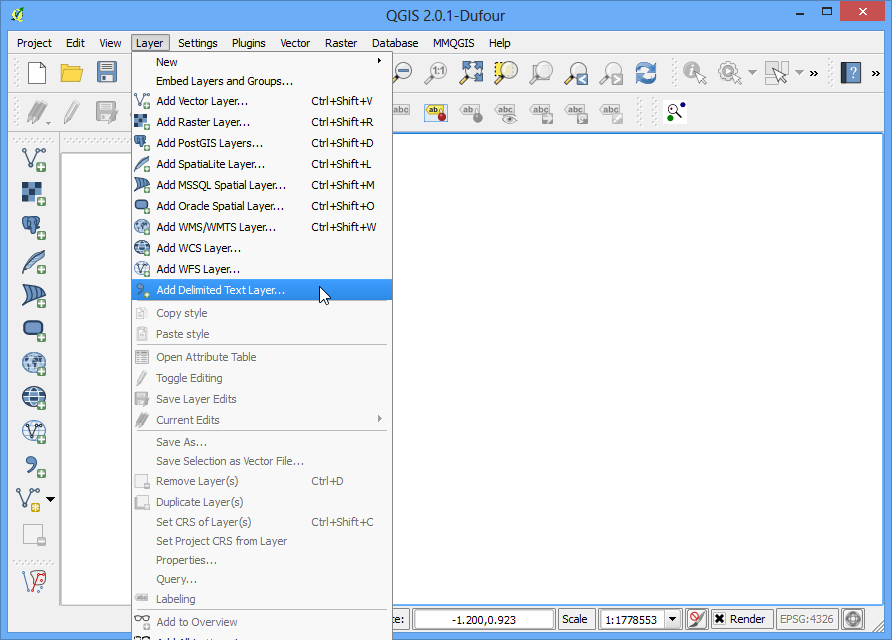
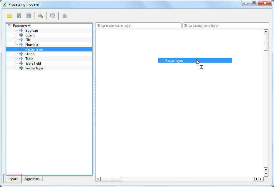
Launch QGIS and go to .
The Processing modeler dialog contains a left-hand panel and a main canvas. Select the Inputs tab in the left-hand panel and drag the + Raster layer to the canvas.
A Parameter definition dialog will pop-up. Enter
Inputas the Parameter name and markYesto Required. Click OK.
You will see a box with the name Input appear in the canvas. This represents the landcover raster that we will use as input. Next step is to apply a
Majority filteralgorithm. Switch to the Algorithm tab from the bottom-left corner. Search for the algorithm and you will find it listed under SAGA provider. Drag it to the canvas.
Opomba
If you do not see this algorithm or any of the subsequent algorithms mentioned in thi tutorial, you may be using the Simplified Interface of the Processing Toolbox. Switch to the Advanced Interface by using the dropdown at the bottom of the Processing Toolbox in the main QGIS window.
A configuration dialog for Majority Filter will be presented. Leave the values to their default and click OK.
You will note that there is now a new box named Majority Filter in the canvas and it is connected to the Input box. This is because the Majority Filter algorithm uses the Input raster as its input. The next step in our workflow is to convert the output of majority filter to vector. Find the
Polygonize (raster to vector)algorithm and drag it to the canvas.
Opomba
The boxes can be moved and arranged by clicking on it and dragging it while holding the left mouse button. You can also use the scroll-wheel to zoom in and out in the model canvas.
Select ‚Filtered Grid‘ from algorithm ‚Majority Filter‘ as the value for Input layer. Click OK.
The final step in the workflow is to query for a class value and create a new layer from the matching features. Search for the
Extract by
attribute
algorithm and drag it the canvas.
Select ‚Vectorized‘ from algorithm ‚Polygonize (raster to vector) as the Input Layer. We want to extract the pixels that represent Croplands. The corresponding pixel value for this class will be 12. (see Code Values). Enter
DNas the Selection attribute and12as the value. As the output of this operation will be the final result, we need to name the output. Entervectorized classas the Output.
Enter the Model name as
vectorizeand Group name asraster. Click the Save button.
Name the model
vectorizeand click Save.
Now it is time to test our model. Close the modeler and switch to the main QGIS window. Go to .
Browse to the downloaded
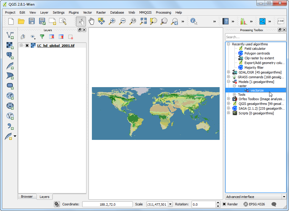
LC_hd_global_2001.tif.gzfile and click Open. Once the raster is loaded, go to .
Find the newly created model under . Double-click to launch the model.
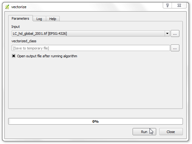
Select
LC_hd_global_2001as the Input and click Run.
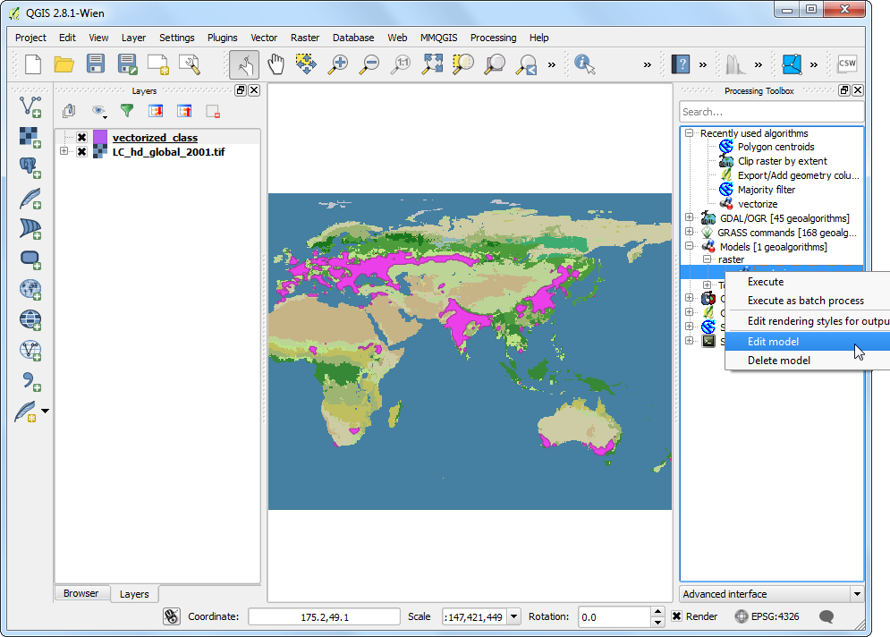
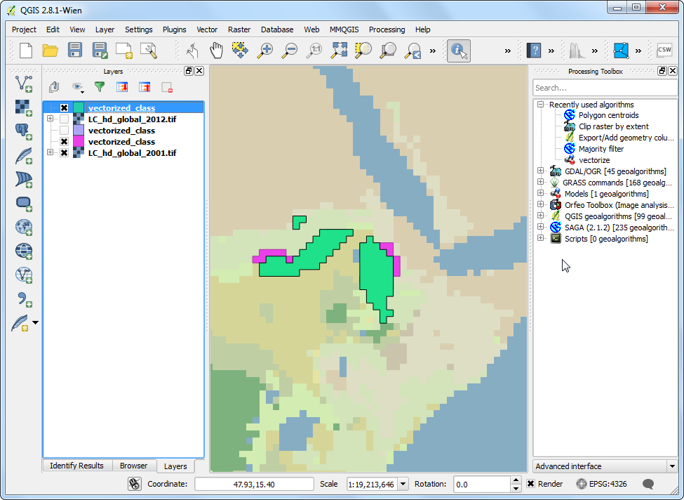
You will see all the steps being executed without any user input. Once the processing finishes, a new layer
vectorized_classwill be added to QGIS. Let’s improve the model a little bit. Right-click on thevectorizemodel and select Edit model.
In Step 12, we hard-coded the value
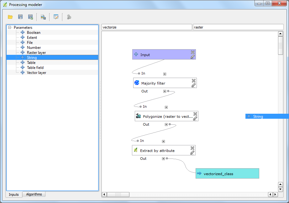
12as the class value. Instead, we can specify it as a input parameter which the user can change. To add this, switch to the Inputs tab and drag the + String to the model.
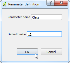
Enter the Parameter Name as
Class. Enter12as the Default value.
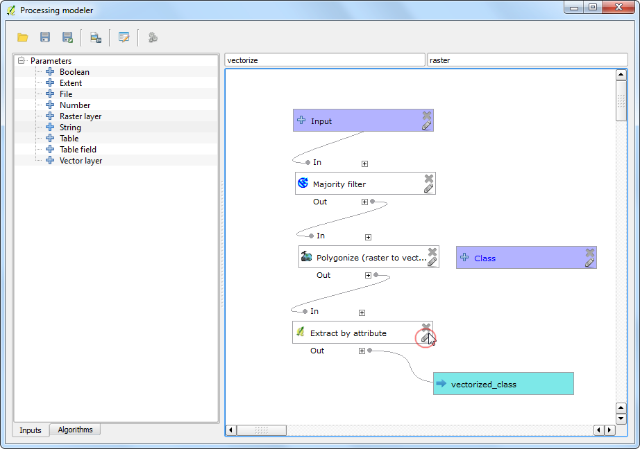
We will now change the
Extract by attributealgorithm to use this input instead of the hard-coded value. Click the Edit button next to the Extract by attribute box.
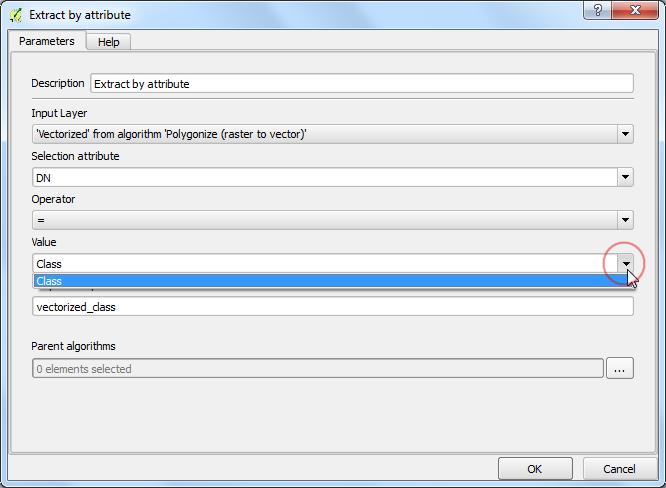
Click the dropdown arrow for Value and select
Class. Click OK.
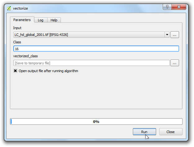
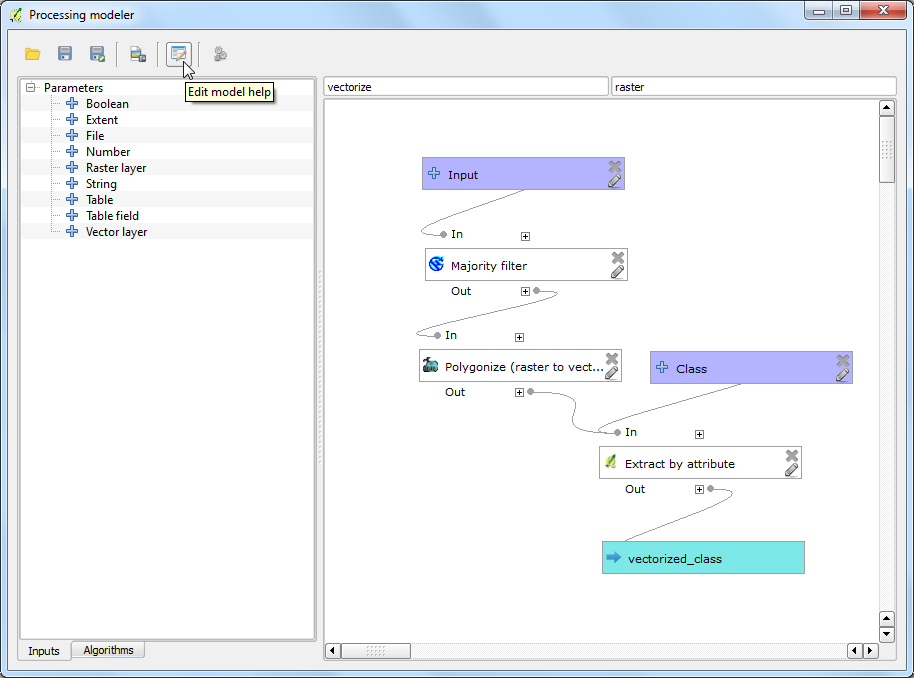
You will see from the model diagram that the Extract by attribute algorithm now uses 2 inputs. The modeler has a shortcut to launch the model and test it. Click the Run button from the toolbar.
Notice that the model dialog has a new editable field called Class. Enter
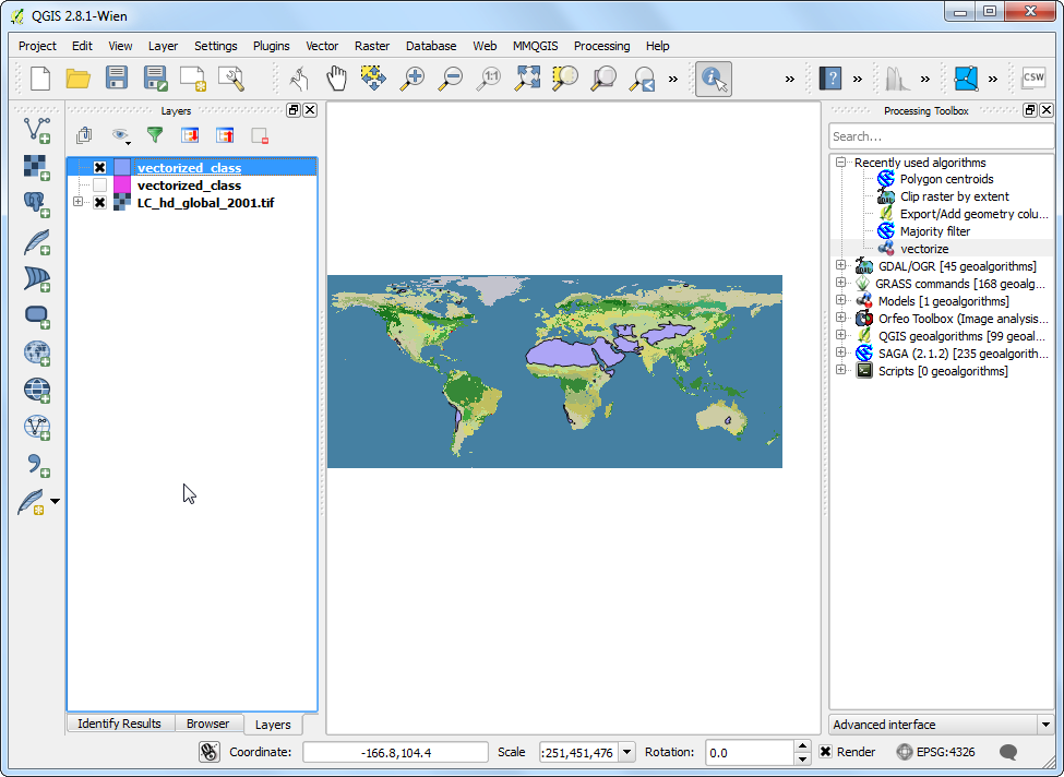
16as the Class value and click Run.
Once the processing finishes, you will see that with just a click of a button we were able to run a complex workflow and extract the area for class 16.
Now that our model is ready, we can run it just as easily on a new raster layer. Load the
LC_hd_global_2012.tif.gzfile by going to . Click the vectorize` model from the Processing Toolbox panel.
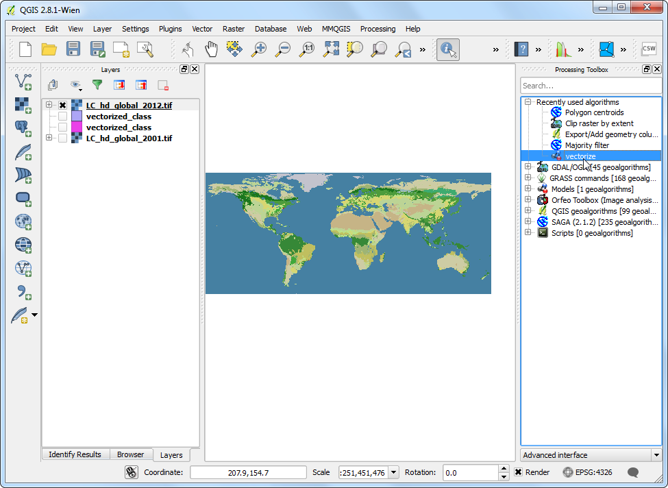
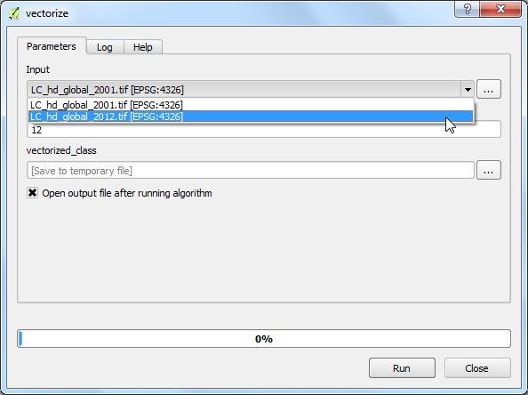
Pick the
LC_hd_global_2012layer as the Input and click Run.
Once the new output is loaded, you can compare the changes in the Croplands from 2001 to 2012.
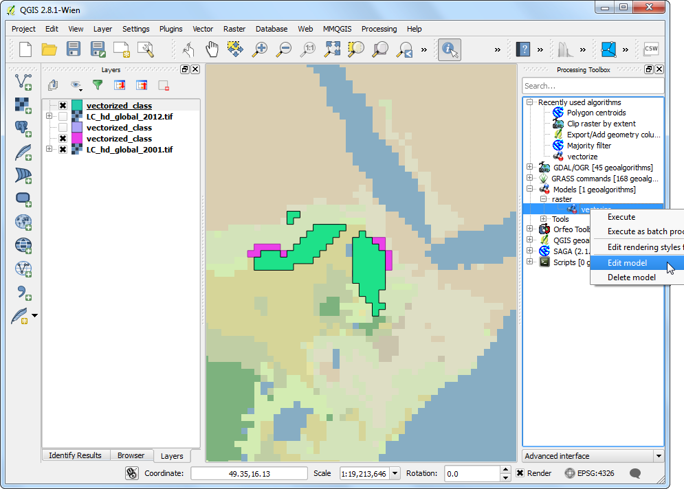
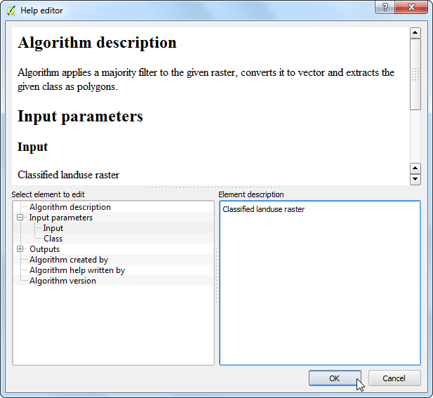
It is always a good idea to add documentation to your model. The modeler has a built-in Help editor that allows you to embed help directly in the model. Right-click the
vectorizemodel and select Edit model.
Click the Edit model help button from the toolbar.
In the Help editor dialog, select any item from the Select element to edit panel and enter the help text in Element description. Click OK. This help will be available in the Help tab when you launch the model to run.
Models can be a great timesaver and allow you to write your workflow once and
run it multiple times. You can even share your model with other users. The
model files are saved in the .qgis2 directory. You can send the .model
file to another user who can copy it to the appropriate directory on their
computer and it will appear in the Processing toolbox. The models
directory location will depend on the platform as follows: (Replace
username with your login name)
Windows
c:\Users\username\.qgis2\processing\models\
Mac
/Users/username/.qgis2/processing/models/
Linux
/home/username/.qgis2/processing/models/
If you want to give feedback or share your experience with this tutorial, please comment below. (requires GitHub account)